Update (12/02/2020): The implementation is now available as a pip package. Simply run pip install torchnca.

While reading related work¹ for my current research project, I stumbled upon a reference to a classic paper from 2004 called Neighbourhood Components Analysis (NCA). After giving it a read, I was instantly charmed by its simplicity and elegance. Long story short, NCA allows you to learn a linear transformation of your data that maximizes k-nearest neighbours performance. By forcing the transformation to be low-rank, NCA will perform dimensionality reduction, leading to vastly reduced storage sizes and search times for kNN! NCA is a very useful algorithm to have in your toolkit – just like PCA – but it’s very rarely mentioned in the wild. In fact, I couldn’t find any tutorial or reference outside of academic papers. This post is an attempt to rectify this.

Figure 1: Visualizing the embedding space of a synthetic dataset as NCA trains.

I’ve implemented NCA in PyTorch with some added bells and whistles. It took almost 1 week to get it to work right, but I gained a lot of insight along the way. I think implementing algorithms from scratch is a great way of building intuition² for why things work – and by extension when and why they don’t – so I encourage the reader to do the same. There’s also a video presentation of NCA by one of the co-authors on YouTube which should serve as a good supplement to this post.

Paper PyTorch Code

Table of Contents

• kNN: The Good, The Bad, The Ugly
• NCA to the rescue
  • Formulating the loss function
  • NCA as a special case of the contrastive loss
• NCA in PyTorch
  • Initialization
  • Loss function
  • Replacing Conjugate Gradients with SGD
  • Stability tricks
• Boring… Show me what it can do!
  • Dimensionality reduction
  • kNN on MNIST
• Acknowledgements

kNN: The Good, The Bad, The Ugly

Figure 2: kNN's nonlinear decision boundary (source).

You’ve probably heard of k-nearest neighbours (kNN) at least once in your life. It’s one of the first algorithms taught in many machine learning classes, and not without good reason. There’s lots to love about kNN! To name a few:

• It has an extremely simple implementation. In fact, kNN has absolutely no computational training cost.
• It’s decision boundary, controlled by $k$, is highly nonlinear (the lines in Figure 2 are locally linear but their overall shape can’t be defined by a hyperplane). For low values of $k$, kNN has very little inductive bias.
• There’s just a single hyperparameter to tune: the number of neighbours $k$. You can easily find its optimal value with cross-validation.
• It is asymptotically optimal. One can show that as the amount of data approaches infinity, k-NN is guaranteed to yield an error rate no worse than twice the Bayes error rate – the lowest possible error rate for any classifier – on a binary classification task. Or in other words, you can expect the performance of kNN to automatically improve as the number of training examples increases.

But kNN does have some annoying drawbacks that limit its efficiency in big-data regimes. Specifically,

• It has to store and search through the entire training data to classify just one test point. Without any optimizations, test-time classification is roughly $\mathcal{O}(n)$ given $n \gg d$. That’s extremely unappealing from a deployment perspective since we usualy aim for a high test-time efficiency and low memory footprint.
• In high dimensions, it suffers from the curse of dimensionality.
• The choice of the distance metric can have a significant effect on its performance. What then is the optimal distance metric? How should one go about choosing it?

NCA to the Rescue

Rather than having the user specify some arbitrary distance metric, NCA learns it by choosing a parameterized family of quadratic distance metrics, constructing a loss function of the parameters, and optimizing it with gradient descent. Furthermore, the learned distance metric can explicitly be made low-dimensional, solving test-time storage and search issues. How does NCA do this?

It turns out that learning a quadratic distance metric $\mathcal{d}$ of the input space where the performance of kNN is maximized is equivalent to learning a linear transformation $\mathcal{A}$ of the input space, such that in the transformed space, kNN with a Euclidean distance metric is maximized. In fact, quadratic distance metrics³ can be represented by a positive semi-definite matrix $Q = \mathcal{A}^T \mathcal{A}$ such that:

$$\begin{equation} \label{eq1} \begin{split} d(x_1, x_2) &= (x_1 - x_2)^T Q (x_1- x_2) \\ & = (\mathcal{A}x_1 - \mathcal{A}x_2)^T (\mathcal{A}x_1 - \mathcal{A}x_2) \\ &= \langle y_1 - y_2, y_1 - y_2 \rangle \end{split} \end{equation}$$

The goal of the learning algorithm then, is to optimize the performance of kNN on future test data. Since we don’t a priori know the test data, we can choose instead to optimize the closest thing in our toolbox: the leave-one-out (LOO) performance of the training data.

At this point, I’d like the reader to appreciate the elegance of NCA. We’ve transformed the problem of maximizing the classification accuracy of kNN into an optimization problem involving a two-dimensional matrix $\mathcal{A}$. What remains is specifying a loss function that’s parameterized by $\mathcal{A}$ and that can serve as as a proxy for the LOO classification accuracy.

Figure 3: The discontinuous graph of the LOO cross validation error. The red rectangle in particular illustrates how an infinitesimal change in the x-axis may change the value of the y-axis by a finite amount.

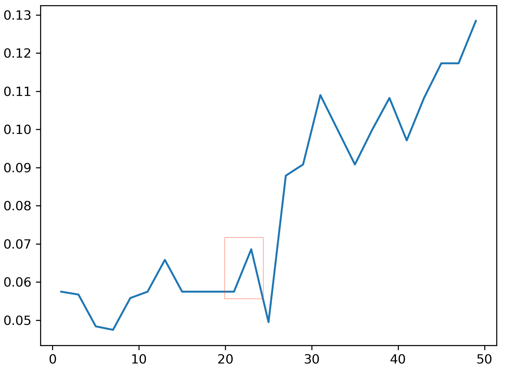
Formulating The Loss Function. There’s a slight bump in our road: LOO error is a highly discontinuous loss function. The reason is that it depends solely on the neighbourhood graph of each point. If the distance metric changes slightly at first, there might be no change in the neighbourhood graph and thus no change of the LOO error. But then suddenly, an infinitesimal change in the metric can alter the neighbourhood graph of many points, causing a significant jump in the LOO error. This is illustrated in the figure above.

Clearly, a discontinuous loss function is terrible for optimzation so we need to construct an alternative that is smooth and differentiable. The key to doing this is to replace fixed neighbourhood selection (i.e. what is done in LOO cross-validation) with stochastic neighbourhood selection. That is, each point $i$ in the training set selects another point $j$ as its neighbor with some probability $p_{ij}$ that is inversely proportional to the Euclidean distance $d_{ij}$ in the transformed space. By summing over all values of $j$, we can compute the probability $p_i$ that a point $i$ will be correctly classified and then sum over all values of $p_i$ to obtain the total number of points we can expect to correctly classifiy.

Denoting the set of points in the same class as $i$ by $C_i$, our loss function⁴ thus becomes:

$$\mathcal{L}(X; \mathcal{A}) = -\sum_i p_i = - \sum_i \sum_{j \in C_i} p_{ij}$$

where

$$\begin{equation} \label{eq2} \begin{split} p_{ij} &= \frac{e^{-d_{ij}}}{\sum_{k \neq i} e^{-d_{ik}}} &= \frac{\exp{\big(-\lVert Ax_i - Ax_j \lVert ^2\big)}}{\sum_{k \neq i} \exp{\big(- \lVert A x_i - Ax_k \lVert}\big)} \end{split} \end{equation}$$

The really neat thing about this stochastic assignment is that we’ve completely avoided having to specify a value of $k$. It gets learned implicitly through the scale of the matrix $\mathcal{A}$:

• With larger values of $\mathcal{A}$, the distance between points increases and as a result their probabilities decrease (think exponential of smaller and smaller values). This means kNN will consult fewer neighbours for each point.
• With smaller values of $\mathcal{A}$, the distance between points decreases and as a result their probabilities increase (think exponential of larger and larger values). This means kNN will consult more neighbours for each point.

NCA as a special case of the contrastive loss. If we slightly alter our loss function to sum over log probabilities $-\sum_i \log{p_i}$, you’ll notice it looks just like a categorical cross entropy loss. In fact, you can think of NCA as a single hidden layer feed-forward neural network that performs metric learning with a contrastive loss function. Recall that a contrastive loss takes on the form:

$$\mathcal{L}_ {contr} = \alpha \mathcal{L}_ {pos} + \beta \mathcal{L}_ {neg}$$

In most papers, $\mathcal{L}_ {pos}$ is an L2 loss, $\mathcal{L}_ {neg}$ is a hinge loss and $\alpha = \beta = 1$. The NCA loss function uses a categorical cross-entropy loss for $\mathcal{L}_ {pos}$ with $\alpha = 1$ and $\beta = 0$. This insight is going to be very valuable in our implementation of NCA when we talk about tricks to stabilize the training.

NCA In PyTorch

There’s currently no GPU-accelerated version of NCA. The two most common ones at the time of this post are sklearn’s python implementation and a C++ implementation. This meant I had the perfect excuse to implement a version in PyTorch that could leverage (a) automatic differentiation to compute the gradient of the loss function with respect to $\mathcal{A}$ and (b) blazing fast GPU acceleration that would prove super useful for large datasets. While the implementation was pretty straightforward, getting it to converge consistently took quite a while. In this section, I’ll walk you through the high-level components needed to implement NCA plus all the additional bells and whistles I added to get it to converge. The entirety of the code is available on GitHub.

Initialization. Since NCA is a gradient-based iterative optimization process, it requires that we specify an initialization strategy for the matrix $\mathcal{A}$. The two obvious ones (no, not zero init!) are identity initialization and random initialization. Recall that if $d$ is the chosen dimension of the embedding space, and if $X \in \mathcal{R}^{N \ \times \ D}$ is our input dataset, then $\mathcal{A} \in \mathcal{R}^{d \ \times \ D}$.

D = 3  # feature space dimension
d = 2  # embedding space dimension

if init == "random":
  # random init from a normal distribution
  # with mean 0 and variance 0.01
  A = nn.Parameter(torch.randn(d, D) * 0.01)
elif init == "identity":
  # identity init
  A = nn.Parameter(torch.eye(d, D))

Loss Function. Computing the loss function requires forming a matrix of pairwise Euclidean distances in the transformed space, applying a softmax over the negative distances to compute pairwise probabilities, then summing over probabilities belonging to the same class. The trick here is to vectorize the softmax computation whilst ignoring diagonal values of the distance matrix (i.e. values where $i = j$) and probabilities that don’t have the same class labels.

To compute a pairwise Euclidean distance matrix, we make use of the following code:

def pairwise_l2_sq(x):
  """Compute pairwise squared Euclidean distances.
  """
  dot = torch.mm(x.double(), torch.t(x.double()))
  norm_sq = torch.diag(dot)
  dist = norm_sq[None, :] - 2*dot + norm_sq[:, None]
  dist = torch.clamp(dist, min=0)  # replace negative values with 0
  return dist.float()

Note the cast to double to increase numerical precision in the dot product computation and the clamp method to replace any negative values that could have arisen from numerical imprecisions with zeros.

Next, we want to compute a softmax over the negative distances to obtain the pairwise probability matrix $p_{ij}$. Unlike a typical softmax implementation, the denominator in our equation sums over all $k \neq i$, i.e. it skips the diagonal entries of the pairwise distance matrix. A neat trick to achieve this without modifying the softmax function is to fill the diagonal entries with np.inf. That way, taking the exponential of their negative evaluates to 0 and doesn’t contribute to the normalization.

Now for each row $i$ in $p_{ij}$, we need to sum over all columns $j \in C_i$. We can achieve this simply by creating a pairwise boolean mask of class labels, element-wise multiplying it with $p_{ij}$ then calling the sum method. The code below executes all the aforementioned computations:

# compute pairwise boolean class label mask
y_mask = (y[:, None] == y[None, :]).float()

# compute pairwise squared Euclidean distances
# in transformed space
embedding = torch.mm(X, torch.t(A))
distances = pairwise_l2_sq(embedding)

# compute pairwise probability matrix p_ij defined by a
# softmax over negative squared distances in the transformed space.
# since we are dealing with negative values with the largest value
# being 0, we need not worry about numerical instabilities
# in the softmax function
p_ij = softmax(-distances)

# for each p_i, zero out any p_ij that is not of the same
# class label as i
p_ij_mask = p_ij * y_mask

# sum over js to compute p_i
p_i = p_ij_mask.sum(dim=1)

# compute expected number of points correctly classified by summing
# over all p_i's.
loss = -p_i.sum()

Replacing Conjugate Gradients with SGD. The authors originally optimized NCA with conjuate gradients. I decided to stick with mini-batch Stochastic Gradient Descent. My reasoning was two-fold. First, with very large datasets, the size of the pairwise matrix grows quadratically with the number of points so it was essential that I use a mini-batch optimizer that could run very fast on a memory-limited GPU. Second, SGD has been shown to be a tried and true optimizer in deep learning that tends to generalize better than its counterparts.

Stability Tricks. It took an intense session of debugging to get the implementation to consistently work for the various initializations and input data sizes. Here they are, in no particular order:

• Summing over log probabilities was more stable than the non-log variant. In other words, I ended up using a categorical cross-entropy loss.
• Initially, the random initialization was sampled from a unit variance Gaussian. Lowering the variance to 0.01 seemed to make the optimization more stable.
• Selecting the batch size was crucial for convergence. A small batch size leads to a very jittery loss function. This makes sense intuitively: a small batch means the pairwise matrix is only a very crude approximation of the neighbourhood graph since it only considers a random subset of all possible neigbhours. I noticed a good rule of thumb was to try to maximize the batch size within the GPU limits.
• Normalizing the input data (i.e. subtracting the mean and dividing by the standard deviation) helped with convergence. Note that doing this requires that we store the computed statistics and scale any test data appropriately.
• Without L2 regularization, the final matrix $\mathcal{A}$ tended to blow up in scale. Adding L2 regularization to the loss function helped tame the matrix and speed-up convergence.
• Random init always converged to a collapsed projection where the points lay on a hyperplane. This is possible because there is no term in the loss function that explicity pulls different classes apart. To combat this, I added a hinge loss component to the loss function, essentially turning the NCA loss into a contrastive loss function.

Boring… Show Me What It Can Do!

At this point, you’re probably curious to know if NCA lives up to its claims. Let’s go ahead and test the PyTorch implementation on 2 tasks: dimensionality reduction and kNN classification.

Using the NCA API is super simple. Very briefly, you first instantiate an NCA object with an embedding dimension and an initialization strategy. Then you call the train method on the input and ground-truth tensors, specifying a batch size and learning rate. There are other parameters you can change, all documented in the class docstring.

nca = NCA(dim=2, init="random")  # instantiate nca object
nca.train(X, y, batch_size=64, lr=1e-4)  # fit nca model
X_nca = nca(X)  # apply the learned transformation

Dimensionality Reduction

For this task, I replicated a portion of the results from section 4 of the paper. Specifically, I generated a synthetic three-dimensional dataset which consists of 5 classes, shown in different colors in Figure 4. The first two dimensions of the dataset correspond to concentric circles, while the third dimension is just Gaussian noise with high variance.

Figure 4: NCA vs. PCA vs. LDA on the synthetic dataset.

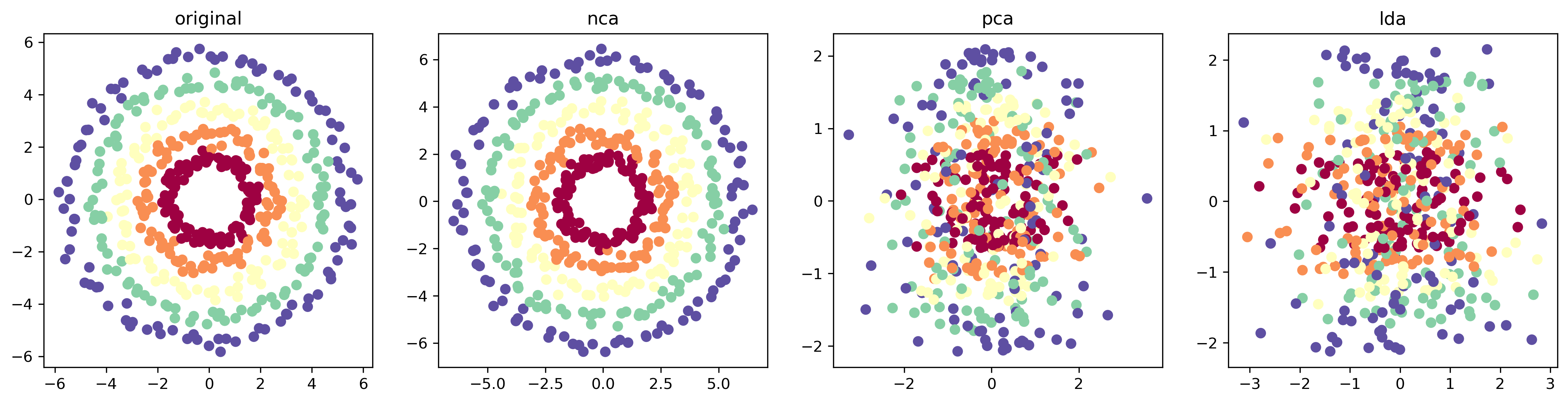
I then embed the dataset to a 2D space using PCA, LDA and NCA. The results are shown Figure 4. While NCA seems to have recovered the original concentric pattern, PCA fails to project out the noise, a direct consequence of the high variance nature of the noise. If we lower it to 0.1 for example, PCA successfully recovers the pattern. LDA also struggles to recover the concentric pattern since the classes themselves are not linearly separable.

kNN On MNIST

The whole motivation for NCA was that it would vastly reduce the storage and search costs of kNN for high-dimensional datasets. To put this to the test, we compared the storage, run time and error rates of two variants of kNN on the MNIST dataset:

• 5-NN on the raw MNIST dataset (784 dimensional)
• 5-NN on the 32 dimensional NCA projection of MNIST

The results are shown in the table below.

Algorithm	Raw kNN	NCA + kNN
Error (%)	2.8	3.3
Time (s)	155.25	2.37
Storage (Mb)	156.8	6.40

That’s a 66x speedup in time and a 25x saveup in storage⁵!

Acknowledgements

I’d like to thank Nick Hynes, Alex Nichol and Brent Yi for their valuable feedback throughout my debugging session and blog writing. I also want to thank Chris Choy for the insight he provided on mode collapse. The javascript code for the animation was adapted from Sam Greydanus’ blog – check him out, he’s got some great content.

---

1. The paper in question is Temporal Cycle Consistency Learning from Dwibedi et. al. ↩

2. John Schulman discusses this in more depth in his latest blog post. ↩

3. You can convince yourself that this is a valid distance metric by checking that the non-negativity, symmetry and triangle inequality conditions are satisfied. ↩

4. We negate the expression because our goal is to maximize the expectation and we’re going to feed it to an optimizer that performs minimization. ↩

5. Performance on MNIST isn’t very representative of real world performance on tougher datasets but this is still a very cool result. ↩