Voronoi Cell Visualization of Nearest Neighborhoods

This is an in-depth tutorial designed to introduce you to a simple, yet powerful classification algorithm called K-Nearest-Neighbors (KNN). We will go over the intuition and mathematical detail of the algorithm, apply it to a real-world dataset to see exactly how it works, and gain an intrinsic understanding of its inner-workings by writing it from scratch in code. Finally, we will explore ways in which we can improve the algorithm.

For the full code that appears on this page, visit my Github Repository.

Table of Contents

1. Introduction
2. What is KNN?
3. How does KNN work?
4. More on K
5. Exploring KNN in Code
6. Parameter Tuning with Cross Validation
7. Writing our Own KNN from Scratch
8. Pros and Cons of KNN
9. Improvements
10. Tutorial Summary

Introduction

The KNN algorithm is a robust and versatile classifier that is often used as a benchmark for more complex classifiers such as Artificial Neural Networks (ANN) and Support Vector Machines (SVM). Despite its simplicity, KNN can outperform more powerful classifiers and is used in a variety of applications such as economic forecasting, data compression and genetics. For example, KNN was leveraged in a 2006 study of functional genomics for the assignment of genes based on their expression profiles.

What is KNN?

Let’s first start by establishing some definitions and notations. We will use $x$ to denote a feature (aka. predictor, attribute) and $y$ to denote the target (aka. label, class) we are trying to predict.

KNN falls in the supervised learning family of algorithms. Informally, this means that we are given a labelled dataset consiting of training observations $(x,y)$ and would like to capture the relationship between $x$ and $y$. More formally, our goal is to learn a function $h : X → Y$ so that given an unseen observation $x$, $h(x)$ can confidently predict the corresponding output $y$.

The KNN classifier is also a non parametric and instance-based learning algorithm.

• Non-parametric means it makes no explicit assumptions about the functional form of h, avoiding the dangers of mismodeling the underlying distribution of the data. For example, suppose our data is highly non-Gaussian but the learning model we choose assumes a Gaussian form. In that case, our algorithm would make extremely poor predictions.
• Instance-based learning means that our algorithm doesn’t explicitly learn a model. Instead, it chooses to memorize the training instances which are subsequently used as “knowledge” for the prediction phase. Concretely, this means that only when a query to our database is made (i.e. when we ask it to predict a label given an input), will the algorithm use the training instances to spit out an answer.

KNN is non-parametric, instance-based and used in a supervised learning setting.

It is worth noting that the minimal training phase of KNN comes both at a memory cost, since we must store a potentially huge data set, as well as a computational cost during test time since classifying a given observation requires a run down of the whole data set. Practically speaking, this is undesirable since we usually want fast responses.

Minimal training but expensive testing.

How does KNN work?

In the classification setting, the K-nearest neighbor algorithm essentially boils down to forming a majority vote between the K most similar instances to a given “unseen” observation. Similarity is defined according to a distance metric between two data points. A popular choice is the Euclidean distance given by

$$d(x, x') = \sqrt{\left(x_1 - x'_1 \right)^2 + \dotsc + \left(x_n - x'_n \right)^2}$$

but other measures can be more suitable for a given setting and include the Manhattan, Chebyshev and Hamming distance.

More formally, given a positive integer K, an unseen observation $x$ and a similarity metric $d$, KNN classifier performs the following two steps:

• It runs through the whole dataset computing $d$ between $x$ and each training observation. We’ll call the K points in the training data that are closest to $x$ the set $\mathcal{A}$. Note that K is usually odd to prevent tie situations.

• It then estimates the conditional probability for each class, that is, the fraction of points in $\mathcal{A}$ with that given class label. (Note $I(x)$ is the indicator function which evaluates to $1$ when the argument $x$ is true and $0$ otherwise)

$$P(y = j | X = x) = \frac{1}{K} \sum_{i \in \mathcal{A}} I(y^{(i)} = j)$$

Finally, our input $x$ gets assigned to the class with the largest probability.

KNN searches the memorized training observations for the K instances that most closely resemble the new instance and assigns to it the their most common class.

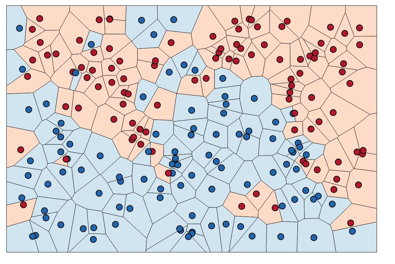
An alternate way of understanding KNN is by thinking about it as calculating a decision boundary (i.e. boundaries for more than 2 classes) which is then used to classify new points.

More on K

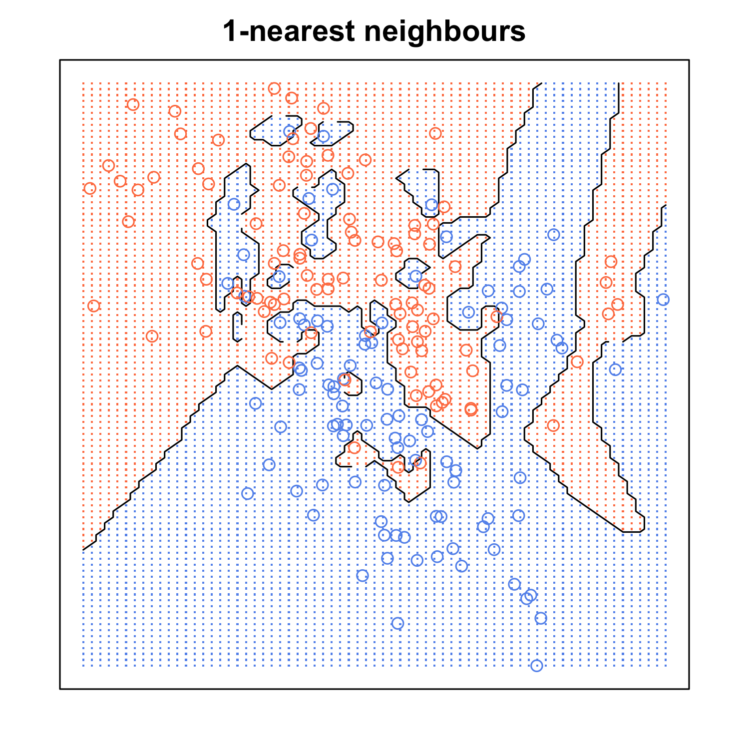
At this point, you’re probably wondering how to pick the variable K and what its effects are on your classifier. Well, like most machine learning algorithms, the K in KNN is a hyperparameter that you, as a designer, must pick in order to get the best possible fit for the data set. Intuitively, you can think of K as controlling the shape of the decision boundary we talked about earlier.

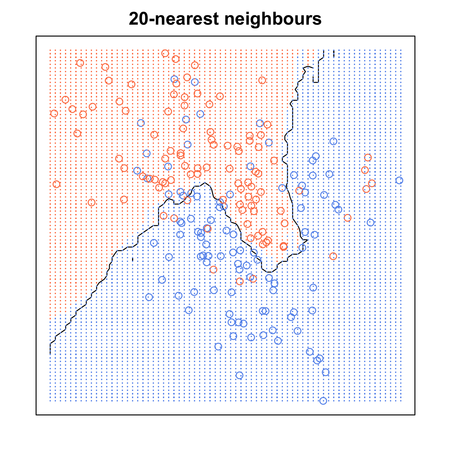
When K is small, we are restraining the region of a given prediction and forcing our classifier to be “more blind” to the overall distribution. A small value for K provides the most flexible fit, which will have low bias but high variance. Graphically, our decision boundary will be more jagged. On the other hand, a higher K averages more voters in each prediction and hence is more resilient to outliers. Larger values of K will have smoother decision boundaries which means lower variance but increased bias.

(If you want to learn more about the bias-variance tradeoff, check out Scott Roe’s Blog post. You can mess around with the value of K and watch the decision boundary change!)

Exploring KNN in Code

Without further ado, let’s see how KNN can be leveraged in Python for a classification problem. We’re gonna head over to the UC Irvine Machine Learning Repository, an amazing source for a variety of free and interesting data sets.

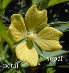
The data set we’ll be using is the Iris Flower Dataset (IFD) which was first introduced in 1936 by the famous statistician Ronald Fisher and consists of 50 observations from each of three species of Iris (Iris setosa, Iris virginica and Iris versicolor). Four features were measured from each sample: the length and the width of the sepals and petals. Our goal is to train the KNN algorithm to be able to distinguish the species from one another given the measurements of the 4 features.

Go ahead and Download Data Folder > iris.data and save it in the directory of your choice.

The first thing we need to do is load the data set. It is in CSV format without a header line so we’ll use pandas’ read_csv function.

import pandas as pd

# define column names
names = [
  'sepal_length',
  'sepal_width',
  'petal_length',
  'petal_width',
  'class',
]

# load training data
df = pd.read_csv('path/iris.data.txt', header=None, names=names)
df.head()

It’s always a good idea to df.head() to see how the first few rows of the data frame look like. Also, note that you should replace 'path/iris.data.txt' with that of the directory where you saved the data set.

Next, it would be cool if we could plot the data before rushing into classification so that we can have a deeper understanding of the problem at hand. R has a beautiful visualization tool called ggplot2 that we will use to create 2 quick scatter plots of sepal width vs sepal length and petal width vs petal length.

# loading packages
library(ggplot2)
library(magrittr)

# sepal width vs. sepal length
iris %>%
  ggplot(aes(x=Sepal.Length, y=Sepal.Width, color=Species)) +
  geom_point()

# petal width vs. petal length
iris %>%
  ggplot(aes(x=Petal.Length, y=Petal.Width, color=Species)) +
  geom_point()

Note that we’ve accessed the iris dataframe which comes preloaded in R by default.

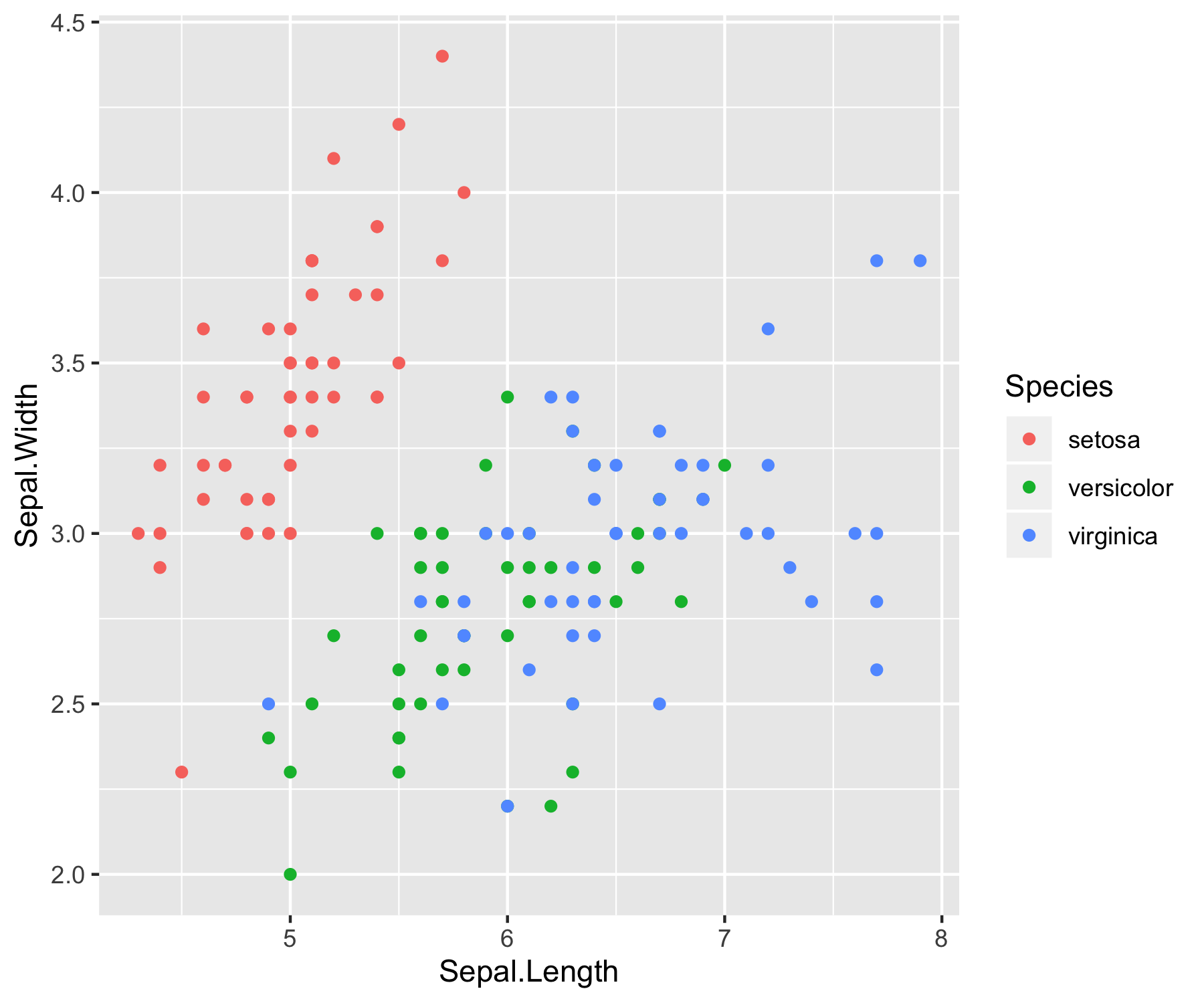
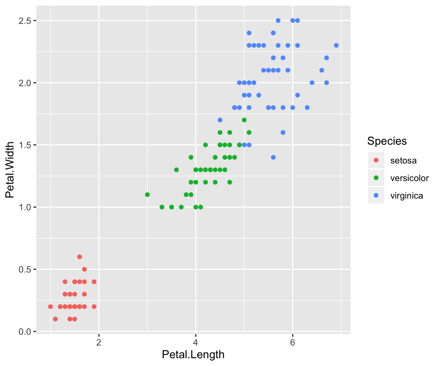
A quick study of the above graphs reveals some strong classification criterion. We observe that setosas have small petals, versicolor have medium sized petals and virginica have the largest petals. Furthermore, setosas seem to have shorter and wider sepals than the other two classes. Pretty interesting right? Without even using an algorithm, we’ve managed to intuitively construct a classifier that can perform pretty well on the dataset.

Now, it’s time to get our hands wet. We’ll be using scikit-learn to train a KNN classifier and evaluate its performance on the data set using the 4 step modeling pattern:

1. Import the learning algorithm
2. Instantiate the model
3. Learn the model
4. Predict the response

scikit-learn requires that the design matrix $X$ and target vector $y$ be numpy arrays so let’s oblige. Furthermore, we need to split our data into training and test sets. The following code does just that.

import numpy as np

from sklearn.cross_validation import train_test_split

# create design matrix X and target vector y
X = np.array(df.ix[:, 0:4])  # end index is exclusive
y = np.array(df['class'])    # another way of indexing a pandas df

# split into train and test
X_train, \
X_test, \
y_train, \
y_test = train_test_split(X, y, test_size=0.33, random_state=42)

Finally, following the above modeling pattern, we define our classifer, in this case KNN, fit it to our training data and evaluate its accuracy. We’ll be using an arbitrary K but we will see later on how cross validation can be used to find its optimal value.

from sklearn.neighbors import KNeighborsClassifier
from sklearn.metrics import accuracy_score

# instantiate learning model (k = 3)
knn = KNeighborsClassifier(n_neighbors=3)

# fitting the model
knn.fit(X_train, y_train)

# predict the response
pred = knn.predict(X_test)

# evaluate accuracy
print("accuracy: {}".format(accuracy_score(y_test, pred)))

Parameter Tuning with Cross Validation

In this section, we’ll explore a method that can be used to tune the hyperparameter K.

Obviously, the best K is the one that corresponds to the lowest test error rate, so let’s suppose we carry out repeated measurements of the test error for different values of K. Inadvertently, what we are doing is using the test set as a training set! This means that we are underestimating the true error rate since our model has been forced to fit the test set in the best possible manner. Our model is then incapable of generalizing to newer observations, a process known as overfitting. Hence, touching the test set is out of the question and must only be done at the very end of our pipeline.

Using the test set for hyperparameter tuning can lead to overfitting.

An alternative and smarter approach involves estimating the test error rate by holding out a subset of the training set from the fitting process. This subset, called the validation set, can be used to select the appropriate level of flexibility of our algorithm! There are different validation approaches that are used in practice, and we will be exploring one of the more popular ones called k-fold cross validation.

K-Fold Cross Validation

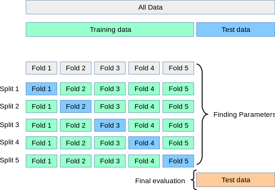
As seen in the image, k-fold cross validation (the k is totally unrelated to K) involves randomly dividing the training set into k groups, or folds, of approximately equal size. The first fold is treated as a validation set, and the method is fit on the remaining $k − 1$ folds. The misclassification rate is then computed on the observations in the held-out fold. This procedure is repeated k times; each time, a different group of observations is treated as a validation set. This process results in k estimates of the test error which are then averaged out.

Cross-validation can be used to estimate the test error associated with a learning method in order to evaluate its performance, or to select the appropriate level of flexibility.

If that is a bit overwhelming for you, don’t worry about it. We’re gonna make it clearer by performing a 10-fold cross validation on our dataset using a generated list of odd K’s ranging from 1 to 50.

# creating odd list of K for KNN
neighbors = list(range(1, 50, 2))

# empty list that will hold cv scores
cv_scores = []

# perform 10-fold cross validation
for k in neighbors:
    knn = KNeighborsClassifier(n_neighbors=k)
    scores = cross_val_score(knn, X_train, y_train, cv=10, scoring='accuracy')
    cv_scores.append(scores.mean())

Again, scikit-learn comes in handy with its cross_val_score method. We specifiy that we are performing 10 folds with the cv = 10 parameter and that our scoring metric should be accuracy since we are in a classification setting.

Finally, we plot the misclassification error versus K.

# changing to misclassification error
mse = [1 - x for x in cv_scores]

# determining best k
optimal_k = neighbors[mse.index(min(mse))]
print("The optimal number of neighbors is {}".format(optimal_k))

# plot misclassification error vs k
plt.plot(neighbors, mse)
plt.xlabel("Number of Neighbors K")
plt.ylabel("Misclassification Error")
plt.show()

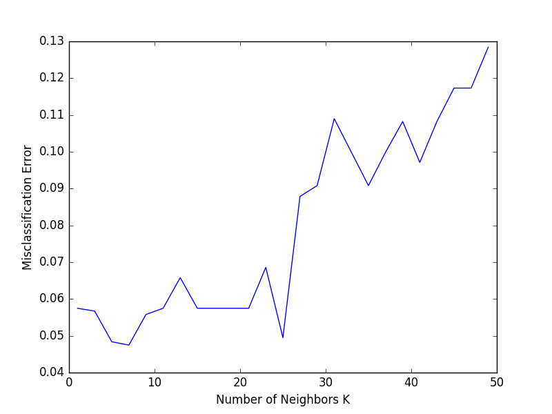
10-fold cross validation tells us that $K = 7$ results in the lowest validation error.

Writing our Own KNN from Scratch

So far, we’ve studied how KNN works and seen how we can use it for a classification task using scikit-learn’s generic pipeline (i.e. input, instantiate, train, predict and evaluate). Now, it’s time to delve deeper into KNN by trying to code it ourselves from scratch.

A machine learning algorithm usually consists of 2 main blocks:

• a training block that takes as input the training data $X$ and the corresponding target $y$ and outputs a learned model $h$.

• a predict block that takes as input new and unseen observations and uses the function $h$ to output their corresponding responses.

In the case of KNN, which as discussed earlier, is a lazy algorithm, the training block reduces to just memorizing the training data. Let’s go ahead a write a python method that does so.

def train(X_train, y_train):
    # do nothing
    return

Gosh, that was hard! Now we need to write the predict method which must do the following: it needs to compute the euclidean distance between the “new” observation and all the data points in the training set. It must then select the K nearest ones and perform a majority vote. It then assigns the corresponding label to the observation. Let’s go ahead and write that.

def predict(X_train, y_train, x_test, k):
    # create list for distances and targets
    distances = []
    targets = []

    for i in range(len(X_train)):
        # compute and store L2 distance
        distances.append([np.sqrt(np.sum(np.square(x_test - X_train[i, :]))), i])

    # sort the list
    distances = sorted(distances)

    # make a list of the k neighbors' targets
    for i in range(k):
        index = distances[i][1]
        targets.append(y_train[index])

    # return most common target
    return Counter(targets).most_common(1)[0][0]

In the above code, we create an array of distances which we sort by increasing order. That way, we can grab the K nearest neighbors (first K distances), get their associated labels which we store in the targets array, and finally perform a majority vote using a Counter.

Putting it all together, we can define the function k_nearest_neighbor, which loops over every test example and makes a prediction.

def k_nearest_neighbor(X_train, y_train, X_test, k):
    # train on the input data
    train(X_train, y_train)

    # loop over all observations
    predictions = []
    for i in range(len(X_test)):
        predictions.append(predict(X_train, y_train, X_test[i, :], k))

    return np.asarray(predictions)

Let’s go ahead and run our algorithm with the optimal K we found using cross-validation.

# making our predictions
predictions = k_nearest_neighbor(X_train, y_train, X_test, 7)

# evaluating accuracy
accuracy = accuracy_score(y_test, predictions)
print("The accuracy of our classifier is {}".format(100*accuracy))

$98\%$ accuracy! We’re as good as scikit-learn’s algorithm, but definitely less efficient. Now what happens if we rerun the algorithm using a large number of neighbors, like k = 140? We get an IndexError: list index out of range error. In fact, K can’t be arbitrarily large since we can’t have more neighbors than the number of observations in the training data set. We can safeguard against this by sanity checking k with an assert statement:

So let’s fix our code to safeguard against such an error:

def k_nearest_neighbor(X_train, y_train, X_test, predictions, k):
    # check if k larger than n
    assert k <= len(X_train), "[!] k can't be larger than number of samples."

    # train on the input data
    train(X_train, y_train)

	# predict for each testing observation
	for i in range(len(X_test)):
        predictions.append(predict(X_train, y_train, X_test[i, :], k))

That’s it, we’ve just written our first machine learning algorithm from scratch!

Pros and Cons of KNN

Pros. As you can already tell from the previous section, one of the most attractive features of the K-nearest neighbor algorithm is that is simple to understand and easy to implement. With zero to little training time, it can be a useful tool for off-the-bat analysis of some data set you are planning to run more complex algorithms on. Furthermore, KNN works just as easily with multiclass data sets whereas other algorithms are hardcoded for the binary setting. Finally, as we mentioned earlier, the non-parametric nature of KNN gives it an edge in certain settings where the data may be highly “unusual”.

Cons. One of the obvious drawbacks of the KNN algorithm is the computationally expensive testing phase which is impractical in industry settings. Note the rigid dichotomy between KNN and the more sophisticated Neural Network which has a lengthy training phase albeit a very fast testing phase. Furthermore, KNN can suffer from skewed class distributions. For example, if a certain class is very frequent in the training set, it will tend to dominate the majority voting of the new example (large number = more common). Finally, the accuracy of KNN can be severely degraded with high-dimension data because there is little difference between the nearest and farthest neighbor.

Improvements

With that being said, there are many ways in which the KNN algorithm can be improved.

• A simple and effective way to remedy skewed class distributions is by implementing weighed voting. The class of each of the K neighbors is multiplied by a weight proportional to the inverse of the distance from that point to the given test point. This ensures that nearer neighbors contribute more to the final vote than the more distant ones.
• Changing the distance metric for different applications may help improve the accuracy of the algorithm. (i.e. Hamming distance for text classification)
• Rescaling your data makes the distance metric more meaningful. For instance, given 2 features height and weight, an observation such as $x = [180, 70]$ will clearly skew the distance metric in favor of height. One way of fixing this is by column-wise subtracting the mean and dividing by the standard deviation. Scikit-learn’s normalize() method can come in handy.
• Dimensionality reduction techniques like PCA should be executed prior to appplying KNN and help make the distance metric more meaningful.
• Approximate Nearest Neighbor techniques such as using k-d trees to store the training observations can be leveraged to decrease testing time. Note however that these methods tend to perform poorly in high dimensions (20+). Try using locality sensitive hashing (LHS) for higher dimensions.

Tutorial Summary

In this tutorial, we learned about the K-Nearest Neighbor algorithm, how it works and how it can be applied in a classification setting using scikit-learn. We also implemented the algorithm in Python from scratch in such a way that we understand the inner-workings of the algorithm. We even used R to create visualizations to further understand our data. Finally, we explored the pros and cons of KNN and the many improvements that can be made to adapt it to different project settings.

If you want to practice some more with the algorithm, try and run it on the Breast Cancer Wisconsin dataset which you can find in the UC Irvine Machine Learning repository. You’ll need to preprocess the data carefully this time. Do it once with scikit-learn’s algorithm and a second time with our version of the code but try adding the weighted distance implementation.

References

Notes

• Stanfords CS231n notes on KNN. click here
• Wikipedia’s KNN page - click here
• Introduction to Statistical Learning with Applications in R, Chapters 2 and 3 - click here
• Detailed Introduction to KNN - click here

Resources

• Scikit-learn’s documentation for KNN - click here
• Data wrangling and visualization with pandas and matplotlib from Chris Albon - click here
• Intro to machine learning with scikit-learn (Great resource!) - click here

Thank you for reading my guide, and I hope it helps you in theory and in practice!