Learning What to Learn and When to Learn It
Disclaimer: This blog post describes unfinished research and should be treated as a work in progress.
Hello world! I’m coming out of hibernation after 14 months of radio silence on this blog. I have a lot of things to blog about, from my research internship at Stanford University this past summer, to wrapping up my B.Eng. in EE in July – and I’ll hopefully get to those in future blog posts – but today, I’d like to talk about some of the cool research I did in my senior year of undergrad. Unfortunately, it’s not GAN/RL related (read as fortunately) but it’s definitely an interesting aspect of the field that could use some more attention.
The problem we’ll be investigating today is whether we can get Deep Neural Networks (DNNs) to converge faster and learn more efficiently. In particular, we’ll try to answer the following questions:
- Do we really need all the training samples in a dataset to reach a desired accuracy?
- Can we do better than (lazy) uniform sampling of the data in a given training epoch?
It actually turns out that on MNIST, we can reliably speedup training by a factor of 2 using just 30% of the available data1!
Table of Contents
- Motivation
- Refresher
- Quantifying Sample Importance
- Loss Patterns
- SGD on Steroids
- Things I Wish I Tried
- Closing Thoughts
Motivation
Human beings acquire knowledge in a unique way, accelerating their learning by choosing where and when to focus their efforts on the available training material. For example, when practicing a new musical composition, a pianist will spend more time on the difficult measures – breaking them down into manageable pieces that can be progressively mastered – rather than wasting her efforts on the simpler, more familiar parts.
Much of the same can be said about our formal primary and secondary education: our teachers help us learn from a smart selection of examples, leveraging previously acquired concepts to help guide our learning of new tools and abstractions. Human learning thus exhibits resource and time efficiency: we become proficient at mastering new concepts by selecting first, a subset of what is available to us in terms of learning material, and second, the sequence in which to learn the selected items such that we minimize acquisition time.
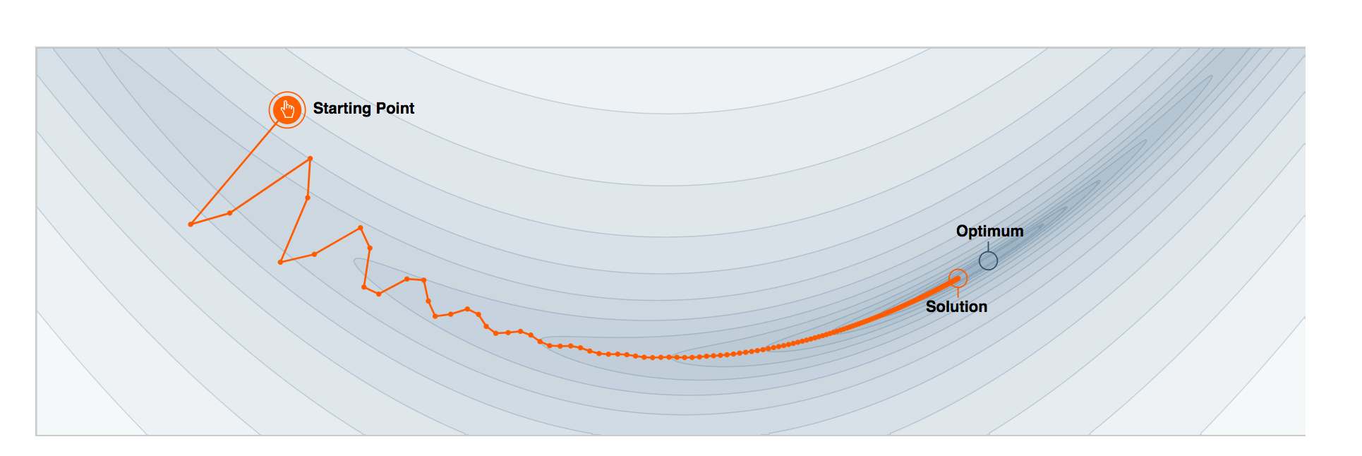
Unfortunately, the training algorithms we use in AI, unlike human learning, are data hungry and time consuming. With vanilla stochastic gradient descent (SGD) for example, the standard go-to optimizer, we repetitively iterate over the training data in sequential mini-batches for a large number of epochs, where a mini-batch is constructed by uniformly sampling training points from the dataset. On large datasets – a necessity for good generalization – the naiveté of this sampling strategy hinders convergence and bottlenecks computation.
Refresher
So how can we improve SGD? Can we replace uniform sampling with a more efficient sampling distribution? More specifically, can we somehow predict a sample’s importance such that we adaptively construct training batches that catalyze more learning-per-iteration? These are all excellent questions we’ll be tackling further in the post, so let’s begin by refreshing a few concepts.
Stochastic Gradient Descent. Given a neural network parameterized by a set of weights , a dataset , and a loss function , we can express the goal of training as finding the optimal set of weights such that,
where corresponds to the number of batches in an epoch, the number of training observations in a batch, and an input-output training pair.
Without loss of generality, we can simplify the notation by considering just one training observation, a special case where the batch size is equal to 1. In that case, training our neural network amounts to updating the weight vector by taking a small step in the direction of the gradient of the loss with respect to between two consecutive iterations:
In the above equation, is a discrete random variable sampled from according to a probability distribution with probabilities and sampling weights . With vanilla SGD and uniform sampling, we have that ,
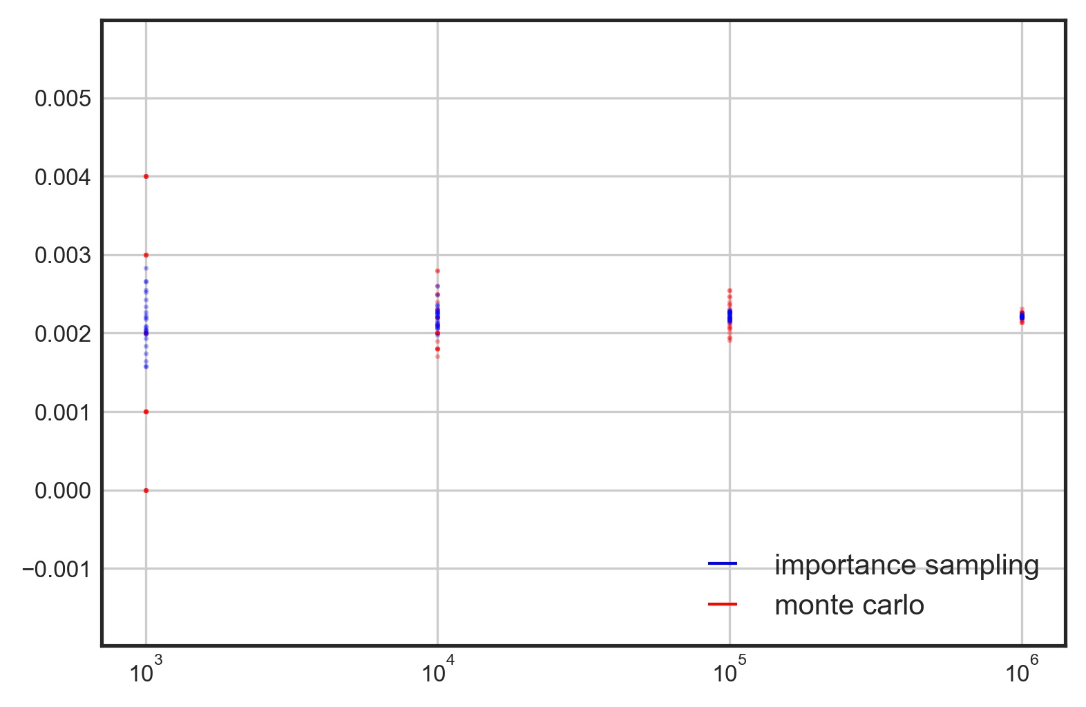
Importance Sampling. Importance sampling is a neat little trick for reducing the variance of an integral estimation by selecting a better distribution from which to sample a random variable. The trick is to multiply the integrand by a cleverly disguised :
Since many quantities of interest (probabilities, sums, integrals)2 can be obtained by computing the mean of a function of a random variable , we can greatly accelerate – and even improve – Monte-Carlo estimates by switching out the original probability distribution with a density that minimizes the sampling of points that contribute very little to the estimate, i.e. points with a function value of 0.
For a tutorial on Monte-Carlo estimation and Importance Sampling, click here.
Quantifying Sample Importance
In the previous section, we mentioned that uniform sampling assigns equal importance to all the training points in . This is obviously wasteful: while some samples are “easy” for the model and can be discarded in the initial stages with minimal impact on performance, the more “difficult” samples should be addressed more frequently throughout the training since they contribute to faster learning. So can we find a way to quantify this “importance”?
Fortunately, the answer is yes: we can theoretically3 show that this quantity is none other than the norm of the gradient of a sample. Intuitively this makes sense: in the classification setting for example, we would expect misclassified examples to exhibit larger gradients than their correctly classified counterparts. Unfortunately, the norm of the gradient is pretty expensive to compute, especially in settings where we would like to avoid computing a full forward and backwards pass.
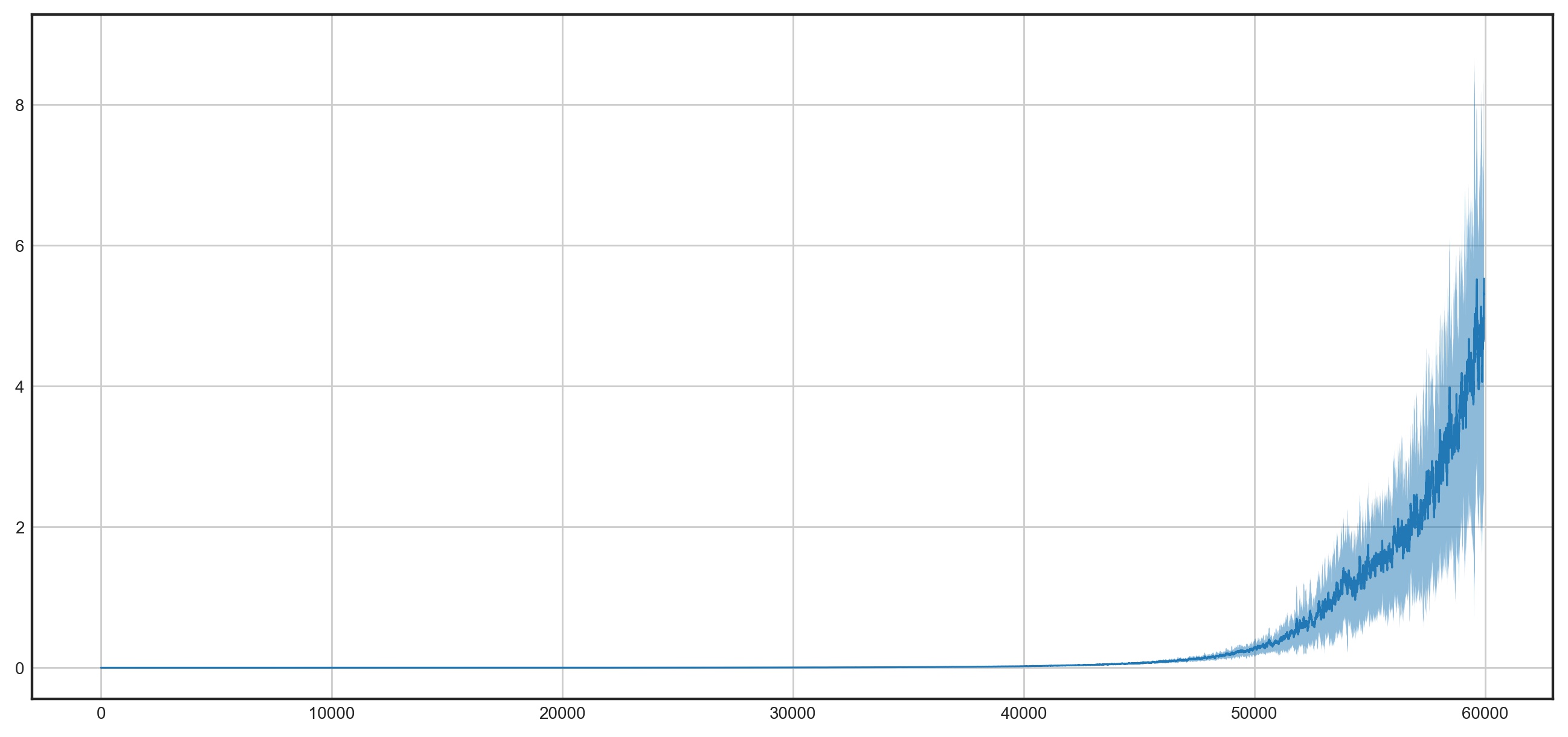
What about the loss of a sample? We essentially get it for free in the forward pass of backprop, so if we can show some degree of correlation with the gradient norm, it would be a less accurate but way cheaper metric for importance. Let’s try and verify this with a small PyTorch experiment. We’re going to train a small convnet on MNIST and record both the loss and gradient of every image in an epoch. We’ll then sort the list containing the gradient norms and use it to index the list of losses. A scatter plot of the reindexed losses should reveal a few things:
- If there is indeed a correlation, there should be a (potentially noisy) straight line through the scatter plot.
- If the correlation is positive – implying that a higher gradient norm corresponds to a higher loss value and vice versa – this line should be increasing.
EDIT (08/06/2019): @AruniRC kindly mentioned that I can compute the Pearson correlation coefficient to numerically quantify the degree of correlation between the gradient norm and the loss value. I’ve now added a cell in the notebook to compute it.
Here’s a code snippet for computing the L2 norm of the gradient of a batch of losses with respect to the parameters of the network. Since there’s a pair of weights and biases associated with every convolutional and fully-connected layer and we want to return a scalar, we can calculate and return the square root of the sum of the squared gradient norms.
def gradient_norm(losses, model):
  norms = []
  for l in losses:
    grad_params = torch.autograd.grad(l, model.parameters(), create_graph=True)
    grad_norm = 0
    for grad in grad_params:
      grad_norm += grad.norm(2).pow(2)
    norms.append(grad_norm.sqrt())
  return norms
Incorporating the above function in the training loop is pretty trivial. All we need to do is record a (grad_norm, loss) tuple for every image in the dataset.
# train for 1 epoch
epoch_stats = []
for batch_idx, (data, target) in enumerate(train_loader):
  data, target = data.to(device), target.to(device)
  optimizer.zero_grad()
  output = model(data)
  losses = F.nll_loss(output, target, reduction='none')
  grad_norms = gradient_norm(losses, model)
  indices = [batch_idx*len(data) + i for i in range(len(data))]
  batch_stats = []
  for i, g, l in zip(indices, grad_norms, losses):
    batch_stats.append([i, [g, l]])
  epoch_stats.append(batch_stats)
  loss = losses.mean()
  loss.backward()
  optimizer.step()
We can compute the correlation between grad_norms and losses using the following one-liner:
corr = np.cov(grad_norms, losses) / (np.std(grad_norms) * np.std(losses))
print("Pearson Correlation Coeff: {}".format(corr[0, 1]))  # prints ~0.83
This returns a value of 0.83 which shows a strong relationship between both variables. Next, we verify this intuition graphically by indexing our losses using the sorted gradient norms and generating the aforementioned scatter plot.
# reindex the losses using the sorted gradient norms
flat = [val for sublist in epoch_stats for val in sublist]
sorted_idx = sorted(range(len(flat)), key=lambda k: flat[k][1][0])
sorted_losses = [flat[idx][1][1].item() for idx in sorted_idx]
The above plot suggests that we can indeed use the loss value of a sample as a proxy for its importance. This is exciting news and opens up some interesting avenues for improving SGD.
If you want to reproduce the above logic, click here.
Loss Patterns
In this section, we’ll try to answer the following question:
Is a sample’s importance consistent across epochs? In other words, if a sample exhibits low loss in the early stages of training, is this still the case in later epochs?
There is substantial benefit in providing empirical evidence to this hypothesis. The reasons are two-fold: first, by eliminating consistently low-loss images from the dataset, we reduce train time proportionally to the discarded images; second, by oversampling the high-loss images, we reduce the variance of the gradients and speedup the convergence to .
To explore this idea, we’re going to track every sample’s loss over a set number of epochs. We’ll bin the loss values into 10 quantiles and compare the histograms over the different epochs. Finally, we’ll repeat these steps with shuffling turned off, then turned on.
NB: We need to be a bit careful with keeping track of a sample’s index when shuffling is turned on. The solution is to create a permutation of [0, 1, 2, ..., 59,999] at the beginning of every epoch and feed it to a sequential sampler with shuffling turned off. By remapping the indices to their true ordering relative to the permutations at the end of training, we would have effectively simulated random shuffling.
If this sounds complicated, let me show you how simple it is to achieve in PyTorch:
# PermSampler takes a list of `indices` and iterates over it sequentially
class PermSampler(Sampler):
  def __init__(self, indices):
    self.indices = indices
  def __iter__(self):
    return iter(self.indices)
  def __len__(self):
    return len(self.indices)

# if `permutation` is None, we return a data loader with no shuffling
# if `permutation` is a list of indices, we return a data loader that iterates
# over the MNIST dataset with indices specified by `permutation`.
def get_data_loader(data_dir, batch_size, permutation=None):
  normalize = transforms.Normalize(mean=(0.1307,), std=(0.3081,))
  transform = transforms.Compose([transforms.ToTensor(), normalize])
  dataset = MNIST(root=data_dir, train=True, download=True, transform=transform)
  sampler = None
  if permutation is not None:
    sampler = PermSampler(permutation)
  loader = DataLoader(dataset, batch_size=batch_size, shuffle=False)
  return loader
After training for 5 epochs, we collect a list containing a tuple (idx, loss_idx) for every image in the dataset. We can remap the indices with the following code:
# remap the indices based on the permutations list
for stat, perm in zip(stats_with_shuffling_flat, permutations):
  for i in range(len(stat)):
    stat[i][0] = perm[i]
Finally, we bin the sorted losses of every epoch into 10 bins and compute the percent match of bins across all epochs, the last 4 epochs, and the last 2 epochs.
def percentage_split(seq, percentages):
  cdf = np.cumsum(percentages)
  assert np.allclose(cdf[-1], 1.0)
  stops = list(map(int, cdf * len(seq)))
  return [seq[a:b] for a, b in zip([0]+stops, stops)]

def bin_losses(all_epochs, num_quantiles=10):
  percentile_splits = []
  for ep in all_epochs:
    sorted_loss_idx = sorted(range(len(ep)), key=lambda k: ep[k][1], reverse=True)
    splits = percentage_split(sorted_loss_idx, [num_quantiles/100]*num_quantiles)
    percentile_splits.append(splits)
  return percentile_splits

fr = [0, 1, 3]
all_matches = []
for f in fr:
  percent_matches = []
  for i in range(num_quantiles):
    percentile_all = []
    for j in range(f, len(percentile_splits)):
      percentile_all.append(percentile_splits[j][i])
      matching = reduce(np.intersect1d, percentile_all)
      percent = 100 * len(matching) / len(percentile_all[0])
      percent_matches.append(percent)
    all_matches.append(percent_matches)
It’s interesting to compute percent matches across a varying range of epochs. The reason is that the training dynamics are less stable in the early epochs when the model weights are still random (analogous to transient response and steady state in circuit theory). For example, we would expect to have higher percent matches if we eliminate the first epoch from the analysis – and this is verified in the below plot!
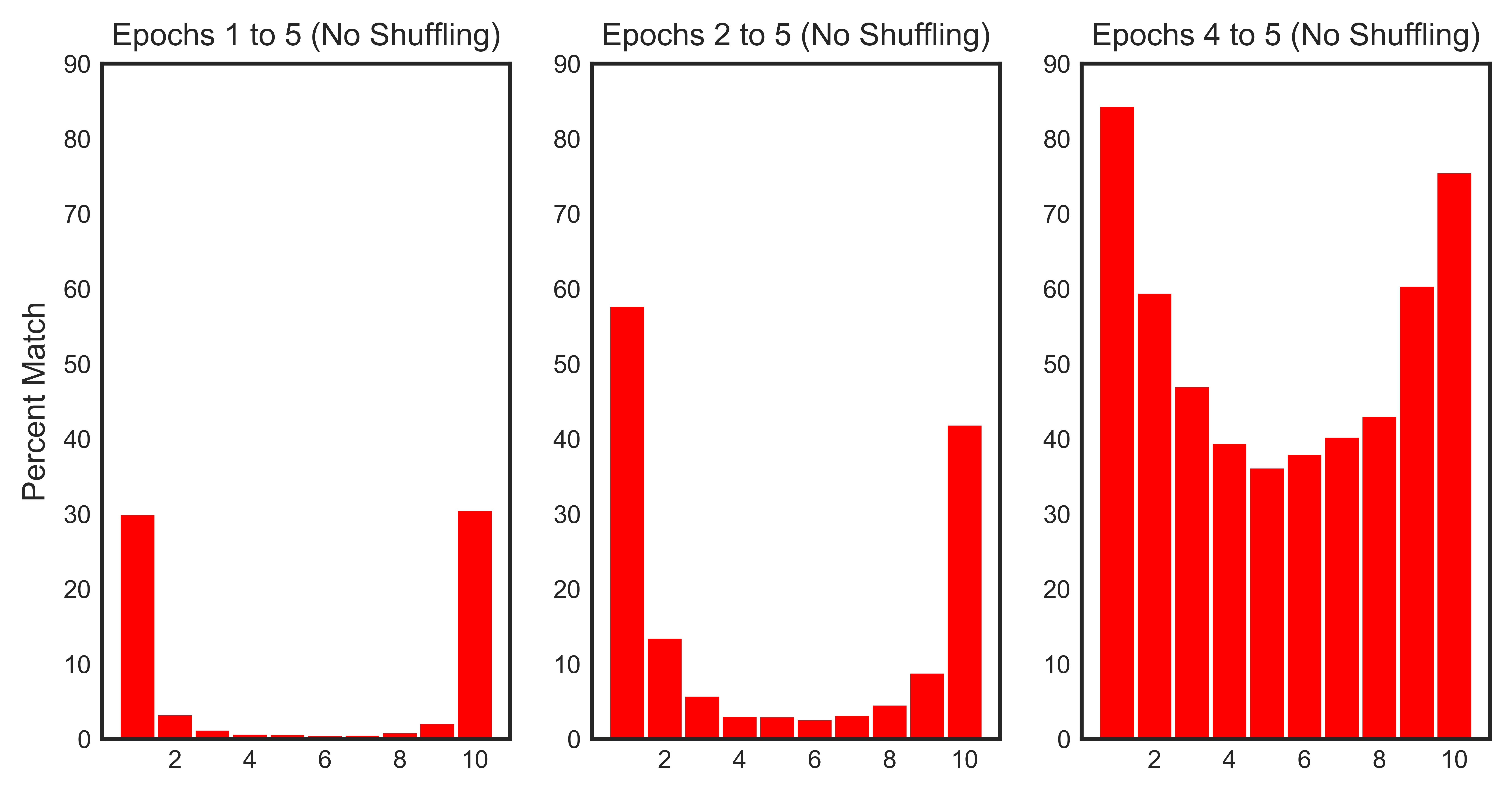
The histograms confirm our hypothesis:
- ~ 30% of the samples with a loss value in the top 10% consistently rank in those ranges across all epochs. This number increases to ~ 60% across epochs 1 through 4 and ~ 85% across the last two epochs.
- ~ 30% of the samples with a loss value in the bottom 10% consistently rank in those ranges across all epochs. This number increases to ~ 50% across epochs 1 through 4 and ~ 70% across the last two epochs.
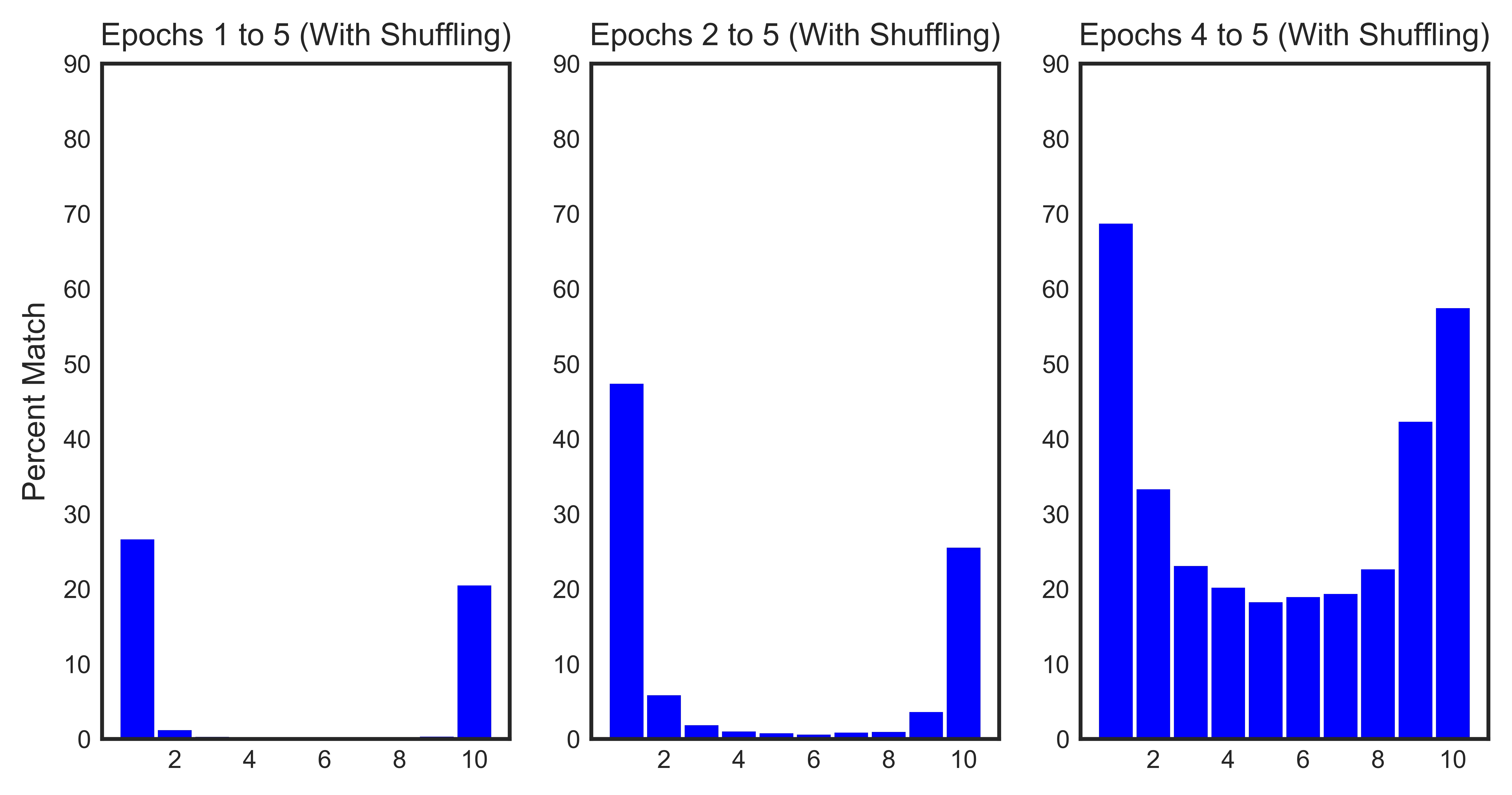
- Shuffling has a minimial impact on the loss evolution of the samples across epochs.
If you want to reproduce the histograms, click here.
SGD on Steroids
Mini-Batch Resampling. In the first version of SGD-S, we’re going to split our training epochs into 2 stages:
- Transient Epochs: in the transient epochs, we train our model exactly as we would in regular SGD. However, in the last epoch, we record and return the losses of every image in the dataset.
- Steady-State Epochs:
- For every epoch in the steady-state, we sample batches using the loss as the sampling distribution.
- At the end of every epoch in the steady-state, we eliminate 10% of the images with the lowest losses. Furthermore, we can choose to randomly introduce a fraction of the discarded images to combat potential catastrophic forgetting.
Let’s illustrate how we can use the loss function to construct an importance sampling distribution for mini-batch resampling. This is achievable using PyTorch’s WeightedRandomSampler in conjunction with the DataLoader.
# sort the loss in decreasing order
sorted_loss_idx = sorted(range(len(losses)), key=lambda k: losses[k][1], reverse=True)

# house cleaning
to_remove = sorted_loss_idx[-int((perc_to_remove / 100) * len(sorted_loss_idx)):]
to_keep = sorted_loss_idx[:-int((perc_to_remove / 100) * len(sorted_loss_idx))]
to_add = list(np.random.choice(removed, int(.01*len(sorted_loss_idx)), replace=False))

new_idx = to_keep + to_add
new_idx.sort()

weights = [losses[idx][1] for idx in new_idx]
sampler = WeightedRandomSampler(weights, len(weights), True)