Understanding Recurrent Neural Networks - Part I
Recurrent Neural Networks have been my Achilles’ heel for the past few months. Admittedly, I haven’t had the grit to sit down and work out their details, but I’ve figured it’s time I stop treating them like black boxes and try instead to discover what makes them tick. My intentions with this series are hence twofold: first, to combat my weakness by understanding their inner workings and coding one from scratch; and second, to write down what I learn in order to reinforce the insights I may gain along the way.
In this first installment, we’ll be introducing the intuition behind RNNs, motivating their use by highlighting a glaring limitation of traditional neural networks. We’ll then transition into a more technical description of their architecture which will be useful for the next installment where we’ll code one from scratch in numpy.
Table of Contents
- Human Learning
- The Woes of Traditional Neural Nets
- Enhancing Neural Networks with Memory
- The Nitty Gritty Details
- References
Human Learning
We are the sum total of our experiences. None of us are the same as we were yesterday, nor will be tomorrow.
B.J. Neblett
There is an inherent truth to the quote above. Our brain pools from past experiences and combines them in intricate ways to solve new and unseen tasks. It is hardwired to work with sequences of information that we perpetually store and call upon over the course of our lives. At its core, human learning can be distilled into two fundamental processes:
- memorization: every time we gain new information, we store it for future reference.
- combination: not all tasks are the same, so we couple our analytical skills with a combination of our memorized, previous experiences to reason about the world.
Consider the following pictures.


Even though it’s in a very weird position, a child can instantly tell that the fur ball in front of it is a cat. It’ll recognize the ears, the whiskers and the snout (memory) but the shape of it all may throw it off. Subconciously however, the child may recall how human stretching deforms shape and pose (combination), and infer that the same is happening to the cat.
Not all tasks require the distant past however. At times, solving a problem makes use of information that was processed only moments ago. For example, take a look at this incomplete sentence:
I bought my usual caramel-covered popcorn with iced tea and headed to the ___.
If I asked you to fill-in the missing word, you’d probably guess “movies”. How did you know that library or starbucks were invalid words? Well, it’s probably because you used context, or information from earlier in the sentence to infer the correct answer. Now think about the following. If I asked you to recite the lyrics of your favorite song backwards, would you be able to do it? Probably not… What about counting backwards? Yeah, piece of cake!
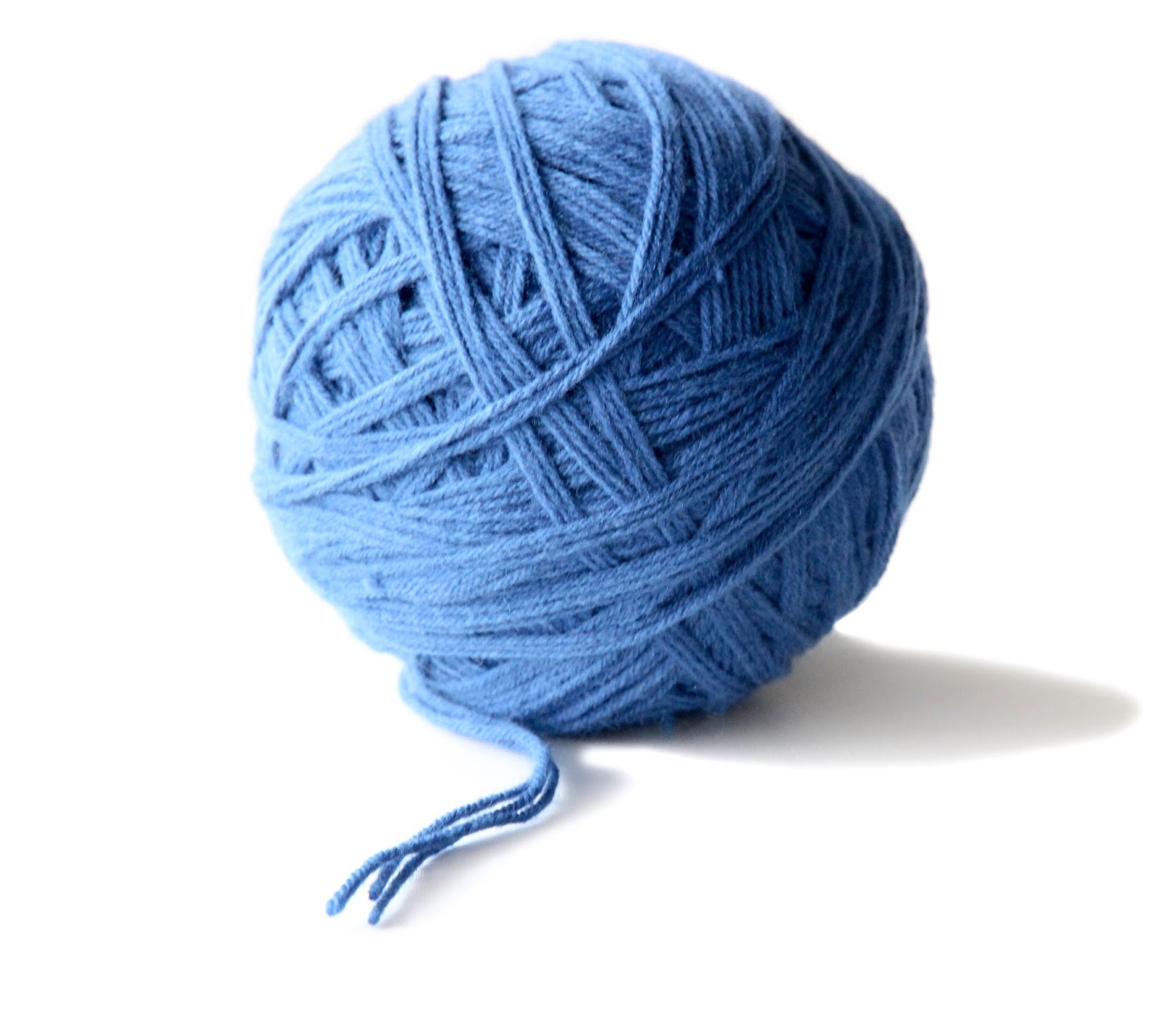
So what makes reciting the song backwards so excruciatingly difficult? The answer is that counting backwards is done on the fly. There is a logical relationship between each number, and knowing the order of the 9 digits and how subtraction works means you can count backwards from say 1845098 even if you’ve never done it before. On the other hand, you memorized the lyrics of the song in a specific order. Your brain works by indexing from one word to the next, starting from the first word. It’s hard to index backwards for the simple reason that your brain has never done it before, so that specific sequence was never stored. Think of the memorized lyric sequence as a giant ball of yarn whose unraveled end can only be accessed with the correct first word in the forward sequence.
The main takeaway is that our brains are naturally talented at working with sequences and they do so by relying on a deceptively simple, yet powerful concept called information persistence.
The Woes of Traditional Neural Nets
We live in a world that is inherently sequential. Audio, video, and language (even your DNA!) are but a few examples of data in which information at a given time step is intricately dependent on information from previous timesteps. So how is all this related to deep learning? Well, think about feeding a sequence of frames from a video into a neural network and asking it to predict what comes next… Or, back to our previous example, feeding a set of words and asking it to complete the sentence.
It should be obvious to you that information from the past is crucial for outputting a sane and plausible prediction. But traditional neural networks can’t do this because they operate on the fundamental assumption that inputs are independent! This is a problem because it means our output at any given time is completely and solely determined by the input at that same time. There is no previous history and our network cannot capitalize on the complex temporal dependencies that exist between the different frames or words to refine its predictions.
This is where Recurrent Neural Networks come in! RNNs allow us to deal with sequences by incorporating a mechanism that stores and leverages information from previous history, sort of like a memory. Put differently, whereas a traditional net maps one input to an output, a recurrent net maps an entire history of previous inputs to each output. If that’s still obscure to you, just think of RNNs as a traditional neural net enhanced with a loop1, one that allows for information to persist across timesteps.
It is important to note that recurrent neural nets aren’t just bound to sequential data in the sense that many problems can be tackled by decomposing them into a series of smaller subproblems. The idea is that instead of burdening our model with predicting an output in one go, we allow it the much easier task of predicting iterative sub-outputs, where each sub-output is an improvement or refinement on the previous step. As an example, a recurrent net2 was used to generate handwritten digits in a sequential fashion, mimicking the way artists refine and reassess their work with brushstrokes.
The idea is that instead of burdening our model with predicting an output in one go, we allow it the much easier task of predicting iterative sub-outputs, where each sub-output is an improvement or refinement on the previous step.
Enhancing Neural Nets with Memory
So how exactly can we endow our networks with the ability to memorize? To answer this question, let’s recall our basic hidden layer neural network, which takes as input a vector X, dot products it with a weight matrix W and applies a nonlinearity. We’ll consider the output y when three successive inputs are fed through the network. Note that the bias term has been eliminated so as to simplify the notation, and I’ve taken the liberty of coloring the equations to make certain patterns stand out.
Given the simple API above, it’s pretty clear that each output is solely determined by its input, i.e. there is no trace of past inputs in the calculation of its value. So let’s alter the API by allowing our hidden layer to use a combination of both the current input and the previous input, and visualize what happens.
Nice! By introducing recurrence into the formula, we’ve managed to obtain a mix of 2 colors in each hidden layer. Intuitively, our network now has a memory depth of 1, equivalent to “seeing” one step backwards in time. Remember though that our goal is to be able to capture information across all previous timesteps, so this does not cut it.
Hmm… What if we feed in a combination of the current input and the previous hidden layer?
Much better! Our layer at each timestep is now a blend of all the colors that have come before it, allowing our network to take into account all its past history when computing its output. This is the power of recurrence in all its glory: creating a loop where information can persist across timesteps.
The Nitty Gritty Details

At its core, an RNN can be represented by an internal, hidden state h that gets updated with every timestep and from which an output y can be optionally derived3. This update behavior is governed by the following equations:
Don’t let the above notation scare you. It’s actually very simple once you dissect it.
- - we’re multiplying the input by a weight matrix . You can think of this dot product as a way for the hidden layer to extract information out of the input.
- - this dot product is allowing the network to extract information from an entire history of past inputs which it will use in conjunction with information gathered from the current input, to compute its output. This is the crucial, self-defining property of RNNs.
- and are activation functions that squash the dot products to a specific range. The function is usually
tanhorReLU. can be asoftmaxwhen we want to output class probabilities. - and are biases that help offset the outputs away from the origin (similar to the b in your typical line).
As you can see, the Vanilla RNN model is quite simple. Once its architecture has been defined, training it is exactly the same as with normal neural nets, i.e. initializing the weight matrices and biases, defining a loss function and minimizing that loss function using some form of gradient descent.
This conclues our first installment in the series. In next week’s blog post, we’ll be coding our very own RNN from the ground up in numpy and apply it to a language modeling task. Stay tuned until then…
References
There are a ton of resources that helped me better grasp the fundamentals of RNNs. I’d like to thank iamtrask especially, for letting me use his idea of colors to explain neural memory. You can read his amazing blog post here.
- Denny Britz’s RNN series - click here
- Andrej Karpathy’s Blog Post - click here
- Chris Olah’s Blog Post - click here
-
If you’re familiar with Control Theory, this should be slightly reminiscent of a feedback loop, although not quite. ↩
-
I’m referring to the DRAW model introduced by Gregor et. al at Deepmind. ↩
-
In the simplest of cases, the hidden state is used as both the output and input to the next hidden state . ↩