Deep Learning Paper Implementations: Spatial Transformer Networks - Part II

In last week’s blog post, we introduced two very important concepts: affine transformations and bilinear interpolation and mentioned that they would prove crucial in understanding Spatial Transformer Networks.
Today, we’ll provide a detailed, section-by-section summary of the Spatial Transformer Networks paper, a concept originally introduced by researchers Max Jaderberg, Karen Simonyan, Andrew Zisserman and Koray Kavukcuoglu of Google Deepmind.
Hopefully, it’ll will give you a clear understanding of the module and prove useful for next week’s blog post where we’ll cover its implementation in Tensorflow.
Table of Contents
Motivation
When working on a classification task, it is usually desirable that our system be robust to input variations. By this, we mean to say that should an input undergo a certain “transformation” so to speak, our classification model should in theory spit out the same class label as before that transformation. A few examples of the “challenges” our image classification model may face include:
- scale variation: variations in size both in the real world and in the image.
- viewpoint variation: different object orientation with respect to the viewer.
- deformation: non rigid bodies can be deformed and twisted in unusual shapes.
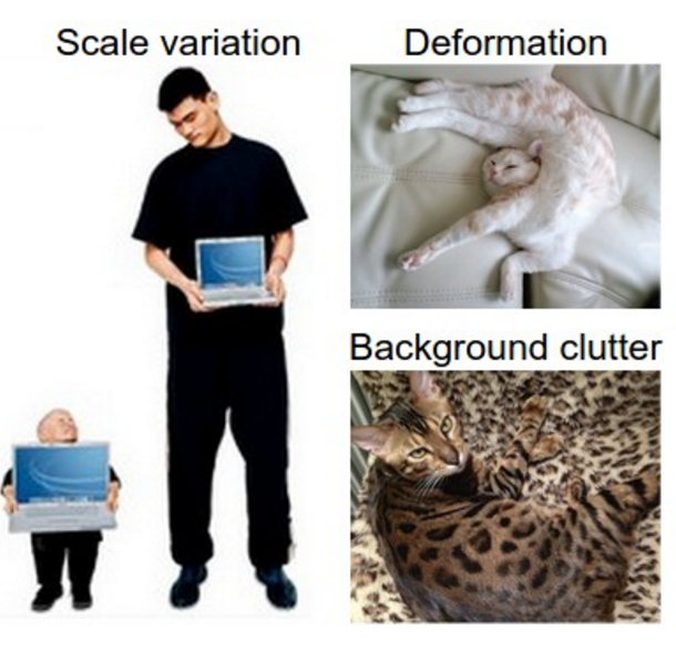
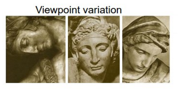
For illustration purposes, take a look at the images above. While the task of classifying them may seem trivial to a human being, recall that our computer algorithms only work with raw 3D arrays of brightness values so a tiny change in an input image can alter every single pixel value in the corresponding array. Hence, our ideal image classification model should in theory be able to disentangle object pose and deformation from texture and shape.
For a different type of intuition, let’s again take a look at the following cat images.

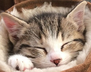


Would it not be extremely desirable if our model could go from left to right using some sort of crop and scale-normalize combination so as to simplify the subsequent classification task?
Pooling Layers
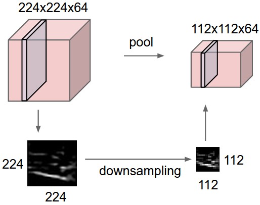
It turns out that the pooling layers we use in our neural network architectures actually endow our models with a certain degree of spatial invariance. Recall that the pooling operator acts as a sort of downsampling mechanism. It progressively reduces the spatial size of the feature map along the depth dimension, cutting down the amount of parameters and computational cost.
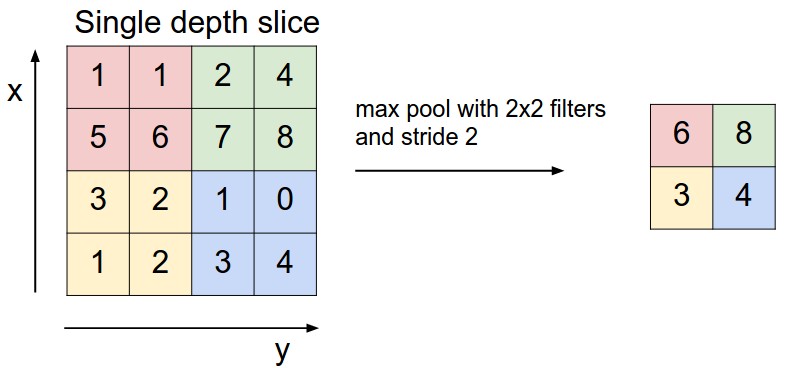
How exactly does it provide invariance? Well think of it this way. The idea behind pooling is to take a complex input, split it up into cells, and “pool” the information from these complex cells to produce a set of simpler cells that describe the output. So for example, say we have 3 images of the number 7, each in a different orientation. A pool over a small grid in each image would detect the number 7 regardless of its position in that grid since we’d be capturing approximately the same information by aggregating pixel values.
Now there are a few downsides to pooling which make it an undesirable operator. For one, pooling is destructive. It discards 75% of feature activations when it is used, meaning we are guaranteed to lose exact positional information. Now you may be wondering why this is bad since we mentioned earlier that it endowed our network with some spatial robustness. Well the thing is that positional information is invaluable in visual recognition tasks. Think of our cat classifier above. It may be important to know where the position of the whiskers are relative to, say the snout. This can’t be achieved when it is this sort of information we throw away when we use max pooling.
Another limitation of pooling is that it is local and predefined. With a small receptive field, the effects of a pooling operator are only felt towards deeper layers of the network meaning intermediate feature maps may suffer from large input distortions. And remember, we can’t just increase the receptive field arbitrarily because then that would downsample our feature map too agressively.
The main takeaway is that ConvNets are not invariant to relatively large input distortions. This limitation is due to having only a restricted, pre-defined pooling mechanism for dealing with spatial variation of the data. This is where Spatial Transformer Networks come into play!
The pooling operation used in convolutional neural networks is a big mistake and the fact that it works so well is a disaster. (Geoffrey Hinton, Reddit AMA)
Spatial Transformer Networks (STNs)
The Spatial Transformer mechanism addresses the issues above by providing Convolutional Neural Networks with explicit spatial transformation capabilities. It possesses 3 defining properties that make it very appealing.
- modular: STNs can be inserted anywhere into existing architectures with relatively small tweaking.
- differentiable: STNs can be trained with backprop allowing for end-to-end training of the models they are injected in.
- dynamic: STNs perform active spatial transformation on a feature map for each input sample as compared to the pooling layer which acted identically for all input samples.
As you can see, the Spatial Transformer is superior to the Pooling operator in all regards. So this begs the following question: what exactly is a Spatial Transformer?
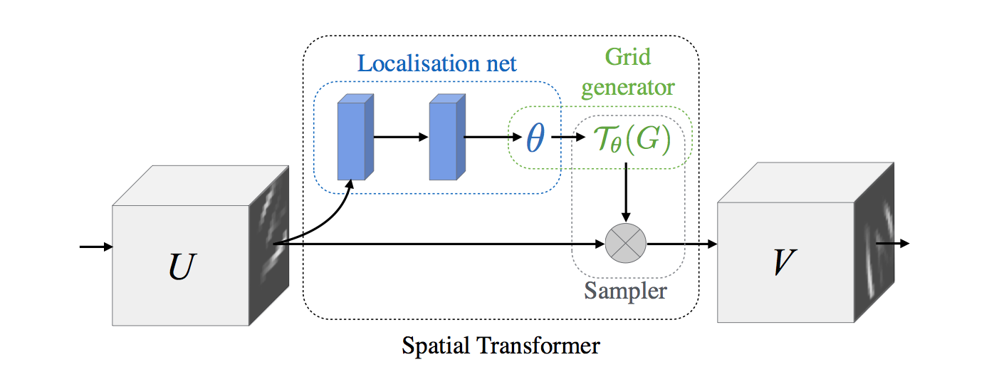
The Spatial Transformer module consists in three components shown in the figure above: a localisation network, a grid generator and a sampler. Before we dive into each of their details, I’d like to briefly remind you of a 3 step pipeline we talked about last week.
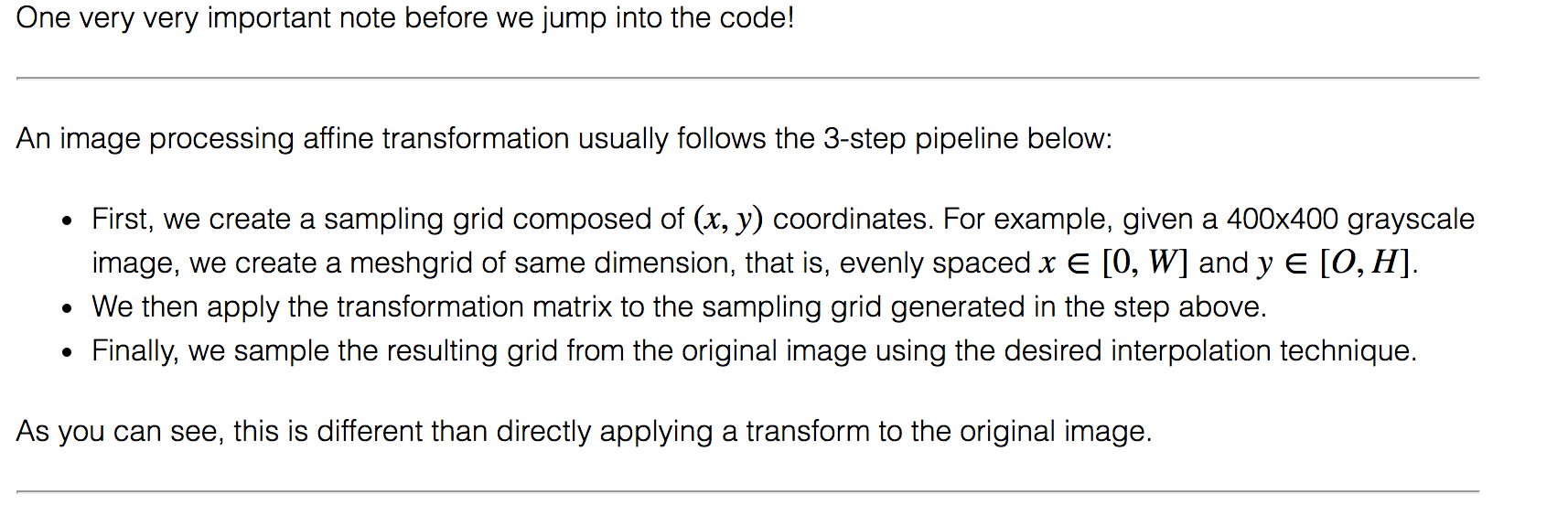
Recall that we can’t just blindly rush to the input image and apply our affine transformation. It’s important to first create a sampling grid, transform it, and then sample the input image using the grid. With that being said, let’s jump into the core components of the Spatial Transformer.
Localisation Network
The goal of the localisation network is to spit out the parameters of the affine transformation that’ll be applied to the input feature map. More formally, our localisation net is defined as follows:
- input: feature map U of shape (H, W, C)
- output: transformation matrix of shape (6,)
- architecture: fully-connected network or ConvNet as well.
As we train our network, we would like our localisation net to output more and more accurate thetas. What do we mean by accurate? Well, think of our digit 7 rotated by 90 degrees counterclockwise. After say 2 epochs, our localisation net may output a transformation matrix which performs a 45 degree clockwise rotation and after 5 epochs for example, it may actually learn to do a complete 90 degree clockwise rotation. The effect is that our output image looks like a standard digit 7, something our neural network has seen in the training data and can easily classify.
Another way to look at it is that the localisation network learns to store the knowledge of how to transform each training sample in the weights of its layers.
Parametrised Sampling Grid
The grid generator’s job is to output a parametrised sampling grid, which is a set of points where the input map should be sampled to produce the desired transformed output.
Concretely, the grid generator first creates a normalized meshgrid of the same size as the input image U of shape (H, W), that is, a set of indices that cover the whole input feature map (the subscript t here stands for target coordinates in the output feature map). Then, since we’re applying an affine transformation to this grid and would like to use translations, we proceed by adding a row of ones to our coordinate vector to obtain its homogeneous equivalent. This is the little trick we also talked about last week. Finally, we reshape our 6 parameter to a 2x3 matrix and perform the following multiplication which results in our desired parametrised sampling grid.
The column vector consists in a set of indices that tell us where we should sample our input to obtain the desired transformed output.
But wait a minute, what if those indices are fractional? Bingo! That’s why we learned about bilinear interpolation and this is exactly what we do next.
Differentiable Image Sampling
Since bilinear interpolation is differentiable, it is perfectly suitable for the task at hand. Armed with the input feature map and our parametrised sampling grid, we proceed with bilinear sampling and obtain our output feature map V of shape (H’, W’, C’). Note that this implies that we can perform downsampling and upsampling by specifying the shape of our sampling grid. (take that pooling!) We definitely aren’t restricted to bilinear sampling, and there are other sampling kernels we can use, but the important takeaway is that it must be differentiable to allow the loss gradients to flow all the way back to our localisation network.
The above illustrates the inner workings of the Spatial Transformer. Basically it boils down to 2 crucial concepts we’ve been talking about all week: an affine transformation followed by bilinear interpolation. Take a moment and admire the elegance of such a mechanism! We’re letting our network learn the optimal affine transformation parameters that will help it ultimately succeed in the classification task all on its own.
Fun with Spatial Transformers
As a final note, I’ll provide 2 examples that illustrate the power of Spatial Transformers. I’ve attached the references for each example at the bottom of the post, so make sure to look those up if they pique your interest.
Distorted MNIST
Here is the result of using a spatial transformer as the first layer of a fully-connected network trained for distorted MNIST digit classification.
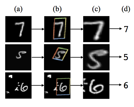
Notice how it has learned to do exactly what we wanted our theoretical “robust” image classification model to do: by zooming in and eliminating background clutter, it has “standardized” the input to facilitate classification. If you want to view a live animation of the transformer in action, click here.
German Traffic Sign Recognition Benchmark (GTSRB) dataset
Summary
In today’s blog post, we went over Google Deepmind’s Spatial Transformer Network paper. We started by introducing the different challenges classification models face, mainly how distortions in the input images can cause our classifiers to fail. One remedy is to use pooling layers; however they possess a few glaring limitations that have made them fall into disuse. The other remedy, and the subject of this blog post, is to use Spatial Transformer Networks.
This consists in a differentiable module that can be inserted anywhere in ConvNet architecture to increase its geometric invariance. It effectively endows our networks with the ability to spatially transform feature maps at no extra data or supervision cost. Finally, we saw how the whole mechanism boils down to 2 familiar operations: an affine transformation and bilinear interpolation.
In next week’s blog post we’ll be using what we’ve learned so far to aid us in coding this paper from scratch in Tensorflow. In the meantime, if you have any questions, feel free to post them in the comment section below.
Cheers and see you next week!