Image Courtesy

I recently sat down to work on assignment 2 of Stanford’s CS231n. It’s lengthy and definitely a step up from the first assignment, but the insight you gain is tremendous.

Anyway, at one point in the assignment, we were tasked with implementing a Batch Normalization layer in our fully-connected net which required writing a forward and backward pass.

The forward pass is relatively simple since it only requires standardizing the input features (zero mean and unit standard deviation). The backwards pass, on the other hand, is a bit more involved. It can be done in 2 different ways:

• staged computation: we can break up the function into several parts, derive local gradients for them, and finally multiply them with the chain rule.
• gradient derivation: basically, you have to do a “pen and paper” derivation of the gradient with respect to the inputs.

It turns out that second option is faster, albeit nastier and after struggling for a few hours, I finally got it to work. This post is mainly a clear summary of the derivation along with my thought process, and I hope it can provide others with the insight and intuition of the chain rule. There is a similar tutorial online already (but I couldn’t follow along very well) so if you want to check it out, head over to Clément Thorey’s Blog.

Finally, I’ve summarized the original research paper and accompanied it with a small numpy implementation which you can view on my Github. With that being said, let’s jump right into the blog.

Notation

Let’s start with some notation.

• BN will stand for Batch Norm.
• $f$ represents a layer upwards of the BN one.
• $y$ is the linear transformation which scales $x$ by $\gamma$ and adds $\beta$.
• $\hat{x}$ is the normalized inputs.
• $\mu$ is the batch mean.
• $\sigma^2$ is the batch variance.

The below table shows you the inputs to each function and will help with the future derivation.

Goal: Find the partial derivatives with respect to the inputs, that is $\dfrac{\partial f}{\partial \gamma}$, $\dfrac{\partial f}{\partial \beta}$ and $\dfrac{\partial f}{\partial x_i}$.

Methodology: derive the gradient with respect to the centered inputs $\hat{x}_i$ (which requires deriving the gradient w.r.t $\mu$ and $\sigma^2$) and then use those to derive one for $x_i$.

Chain Rule Primer

Suppose we’re given a function $u(x, y)$ where $x(r, t)$ and $y(r, t)$. Then to determine the value of $\frac{\partial u}{\partial r}$ and $\frac{\partial u}{\partial t}$ we need to use the chain rule which says that:

$$\frac{\partial u}{\partial r} = \frac{\partial u}{\partial x} \cdot \frac{\partial x}{\partial r} + \frac{\partial u}{\partial y} \cdot \frac{\partial y}{\partial r}$$

That’s basically all there is to it. Using this simple concept can help us solve our problem. We just have to be clear and precise when using it and not get lost with the intermediate variables.

Partial Derivatives

Here’s the gist of BN taken from the paper.

We’re gonna start by traversing the table from left to right. At each step we derive the gradient with respect to the inputs in the cell.

Cell 1

Let’s compute $\dfrac{\partial f}{\partial y_i}$. It actually turns out we don’t need to compute this derivative since we already have it - it’s the upstream derivative dout given to us in the function parameter.

Cell 2

Let’s work on cell 2 now. We note that $y$ is a function of three variables, so let’s compute the gradient with respect to each one.

---

Starting with $\gamma$ and using the chain rule:

$$\begin{eqnarray} \frac{\partial f}{\partial \gamma} &=& \frac{\partial f}{\partial y_i} \cdot \frac{\partial y_i}{\partial \gamma} \qquad \\ &=& \boxed{\sum\limits_{i=1}^m \frac{\partial f}{\partial y_i} \cdot \hat{x}_i} \end{eqnarray}$$

Notice that we sum from $1 \rightarrow m$ because we’re working with batches! If you’re worried you wouldn’t have caught that, think about the dimensions. The gradient with respect to a variable should be of the same size as that same variable so if those two clash, it should tell you you’ve done something wrong.

---

Moving on to $\beta$ we compute the gradient as follows:

$$\begin{eqnarray} \frac{\partial f}{\partial \beta} &=& \frac{\partial f}{\partial y_i} \cdot \frac{\partial y_i}{\partial \beta} \qquad \\ &=& \boxed{\sum\limits_{i=1}^m \frac{\partial f}{\partial y_i}} \end{eqnarray}$$

---

and finally $\hat{x}_i$:

$$\begin{eqnarray} \frac{\partial f}{\partial \hat{x}_i} &=& \frac{\partial f}{\partial y_i} \cdot \frac{\partial y_i}{\partial \hat{x}_i} \qquad \\ &=& \boxed{\frac{\partial f}{\partial y_i} \cdot \gamma} \end{eqnarray}$$

---

Up to now, things are relatively simple and we’ve already done 2/3 of the work. We can’t compute the gradient with respect to $x_i$ just yet though.

Cell 3

---

We start with $\mu$ and notice that $\sigma^2$ is a function of $\mu$, therefore we need to add its contribution to the partial - (I’ve highlighted the missing partials in red):

$$\dfrac{\partial f}{\partial \mu} = \frac{\partial f}{\partial \hat{x}_i} \cdot \color{red}{\frac{\partial \hat{x}_i}{\partial \mu}} + \color{red}{\frac{\partial f}{\partial \sigma^2}} \cdot \color{red}{\frac{\partial \sigma^2}{\partial\mu}}$$

Let’s compute the missing partials one at a time.

From

$$\hat{x}_i = \frac{(x_i - \mu)}{\sqrt{\sigma^2 + \epsilon}}$$

we compute:

$$\boxed{\dfrac{\partial \hat{x}_i}{\partial \mu} = \frac{1}{\sqrt{\sigma^2 + \epsilon}} \cdot (-1)}$$

and from

$$\sigma^2 = \frac{1}{m} \sum\limits_{i=1}^m (x_i - \mu)^2$$

we calculate:

$$\boxed{\dfrac{\partial \sigma^2}{\partial \mu} = \frac{1}{m} \sum\limits_{i=1}^m 2 \cdot (x_i - \mu)\cdot (-1)}$$

We’re missing the partial with respect to $\sigma^2$ and that is our next variable, so let’s get to it and come back and plug it in here.

---

Ok so in the expression of the partial:

$$\begin{eqnarray} \frac{\partial f}{\partial \sigma^2} &=& \frac{\partial f}{\partial \hat{x}} \cdot \frac{\partial \hat{x}}{\partial \sigma^2} \qquad \\ \end{eqnarray}$$

let’s compute $\dfrac{\partial \hat{x}}{\partial \sigma^2}$ in more detail. I’m gonna rewrite $\hat{x}$ to make its derivative easier to compute:

$$\hat{x}_i = (x_i - \mu)(\sigma^2 + \epsilon)^{-0.5}$$

$(x_i - \mu)$ is a constant therefore:

$$\begin{eqnarray} \dfrac{\partial \hat{x}}{\partial \sigma^2} &=& \sum\limits_{i=1}^m (x_i - \mu) \cdot (-0.5) \cdot (\sigma^2 + \epsilon)^{-0.5 - 1} \qquad \\ &=& -0.5 \sum\limits_{i=1}^m (x_i - \mu) \cdot (\sigma^2 + \epsilon)^{-1.5} \end{eqnarray}$$

---

With all that out of the way, let’s plug everything back in our previous partial!

$$\begin{eqnarray} \frac{\partial f}{\partial \mu} &=& \bigg(\sum\limits_{i=1}^m \frac{\partial f}{\partial \hat{x}_i} \cdot \frac{-1}{\sqrt{\sigma^2 + \epsilon}} \bigg) + \bigg( \frac{\partial f}{\partial \sigma^2} \cdot \frac{1}{m} \sum\limits_{i=1}^m -2(x_i - \mu) \bigg) \qquad \\ &=& \bigg(\sum\limits_{i=1}^m \frac{\partial f}{\partial \hat{x}_i} \cdot \frac{-1}{\sqrt{\sigma^2 + \epsilon}} \bigg) + \bigg( \frac{\partial f}{\partial \sigma^2} \cdot (-2) \cdot \bigg( \frac{1}{m} \sum\limits_{i=1}^m x_i - \frac{1}{m} \sum\limits_{i=1}^m \mu \bigg) \bigg) \qquad \\ &=& \bigg(\sum\limits_{i=1}^m \frac{\partial f}{\partial \hat{x}_i} \cdot \frac{-1}{\sqrt{\sigma^2 + \epsilon}} \bigg) + \bigg( \frac{\partial f}{\partial \sigma^2} \cdot (-2) \cdot \bigg( \mu - \frac{m \cdot \mu}{m} \bigg) \bigg) \qquad \\ &=& \sum\limits_{i=1}^m \frac{\partial f}{\partial \hat{x}_i} \cdot \frac{-1}{\sqrt{\sigma^2 + \epsilon}} \qquad \\ \end{eqnarray}$$

Thus we have:

$$\boxed{\frac{\partial f}{\partial \mu} = \sum\limits_{i=1}^m \frac{\partial f}{\partial \hat{x}_i} \cdot \frac{-1}{\sqrt{\sigma^2 + \epsilon}}}$$

---

We finally arrive at the last variable $x$. Again adding the contributions from any parameter containing $x$ we obtain:

$$\dfrac{\partial f}{\partial x_i} = \frac{\partial f}{\partial \hat{x}_i} \cdot \color{red}{\frac{\partial \hat{x}_i}{\partial x_i}} + \frac{\partial f}{\partial \mu} \cdot \color{red}{\frac{\partial \mu}{\partial x_i}} + \frac{\partial f}{\partial \sigma^2} \cdot \color{red}{\frac{\partial \sigma^2}{\partial x_i}}$$

The missing pieces are super easy to compute at this point.

$$\dfrac{\partial \hat{x}_i}{\partial x_i} = \dfrac{1}{\sqrt{\sigma^2 + \epsilon}}$$ $$\dfrac{\partial \mu}{\partial x_i} = \dfrac{1}{m}$$ $$\dfrac{\partial \sigma^2}{\partial x_i} = \dfrac{2(x_i - \mu)}{m}$$

That’s it, our final gradient is

$$\frac{\partial f}{\partial x_i} = \bigg(\frac{\partial f}{\partial \hat{x}_i} \cdot \dfrac{1}{\sqrt{\sigma^2 + \epsilon}}\bigg) + \bigg(\frac{\partial f}{\partial \mu} \cdot \dfrac{1}{m}\bigg) + \bigg(\frac{\partial f}{\partial \sigma^2} \cdot \dfrac{2(x_i - \mu)}{m}\bigg)$$

Note the following trick

$$\boxed{(\sigma^2 + \epsilon)^{-1.5} = (\sigma^2 + \epsilon)^{-0.5}(\sigma^2 + \epsilon)^{-1} = (\sigma^2 + \epsilon)^{-0.5} \frac{1}{\sqrt{\sigma^2 + \epsilon}}\frac{1}{\sqrt{\sigma^2 + \epsilon}}}$$

With that in mind, let’s plug in the partials and see if we can simplify the expression some more.

$$\begin{eqnarray} \frac{\partial f}{\partial x_i} &=& \bigg(\frac{\partial f}{\partial \hat{x}_i} \cdot \dfrac{1}{\sqrt{\sigma^2 + \epsilon}}\bigg) + \bigg(\frac{\partial f}{\partial \mu} \cdot \dfrac{1}{m}\bigg) + \bigg(\frac{\partial f}{\partial \sigma^2} \cdot \dfrac{2(x_i - \mu)}{m}\bigg) \qquad \\ &=& \bigg(\frac{\partial f}{\partial \hat{x}_i} \cdot \dfrac{1}{\sqrt{\sigma^2 + \epsilon}}\bigg) + \bigg(\frac{1}{m} \sum\limits_{j=1}^m \frac{\partial f}{\partial \hat{x}_j} \cdot \frac{-1}{\sqrt{\sigma^2 + \epsilon}}\bigg) - \bigg(0.5 \sum\limits_{j=1}^m \frac{\partial f}{\partial \hat{x}_j} \cdot (x_j - \mu) \cdot (\sigma^2 + \epsilon)^{-1.5} \cdot \dfrac{2(x_i - \mu)}{m} \bigg) \qquad \\ &=& \bigg(\frac{\partial f}{\partial \hat{x}_i} \cdot (\sigma^2 + \epsilon)^{-0.5} \bigg) - \bigg(\frac{(\sigma^2 + \epsilon)^{-0.5}}{m} \sum\limits_{j=1}^m \frac{\partial f}{\partial \hat{x}_j} \bigg) + \bigg(\frac{(\sigma^2 + \epsilon)^{-0.5}}{m} \cdot \frac{x_i - \mu}{\sqrt{\sigma^2 + \epsilon}} \sum\limits_{j=1}^m \frac{\partial f}{\partial \hat{x}_j} \cdot \frac{(x_j - \mu)}{\sqrt{\sigma^2 + \epsilon}} \bigg )\qquad \\ &=& \bigg(\frac{\partial f}{\partial \hat{x}_i} \cdot (\sigma^2 + \epsilon)^{-0.5} \bigg) - \bigg(\frac{(\sigma^2 + \epsilon)^{-0.5}}{m} \sum\limits_{j=1}^m \frac{\partial f}{\partial \hat{x}_j} \bigg) + \bigg(\frac{(\sigma^2 + \epsilon)^{-0.5}}{m} \cdot \hat{x}_i \sum\limits_{j=1}^m \frac{\partial f}{\partial \hat{x}_j} \cdot \hat{x}_j \bigg )\qquad \\ \end{eqnarray}$$

Finally, we factorize by the sigma + epsilon factor and obtain:

$$\boxed{\frac{\partial f}{\partial x_i} = \frac{(\sigma^2 + \epsilon)^{-0.5}}{m} \bigg [\color{red}{m \frac{\partial f}{\partial \hat{x}_i}} - \color{blue}{\sum\limits_{j=1}^m \frac{\partial f}{\partial \hat{x}_j}} - \color{green}{\hat{x}_i \sum\limits_{j=1}^m \frac{\partial f}{\partial \hat{x}_j} \cdot \hat{x}_j}\bigg ]}$$

Recap

For organizational purposes, let’s summarize the main equations we were able to derive. Using $\dfrac{\partial f}{\partial \hat{x}_i} = \dfrac{\partial f}{\partial y_i} \cdot \gamma$, we obtain the gradient with respect to our inputs:

$$\boxed{\color{red}{\frac{\partial f}{\partial \beta} = \sum\limits_{i=1}^m \frac{\partial f}{\partial y_i}}}$$ $$\boxed{\color{blue}{\frac{\partial f}{\partial \gamma} = \sum\limits_{i=1}^m \frac{\partial f}{\partial y_i} \cdot \hat{x}_i}}$$ $$\boxed{\frac{\partial f}{\partial x_i} = \frac{\color{red}{m \dfrac{\partial f}{\partial \hat{x}_i}} - \color{blue}{\sum\limits_{j=1}^m \dfrac{\partial f}{\partial \hat{x}_j}} - \color{green}{\hat{x}_i \sum\limits_{j=1}^m \dfrac{\partial f}{\partial \hat{x}_j} \cdot \hat{x}_j}}{m\sqrt{\sigma^2 + \epsilon}}}$$

Python Implementation

Here’s an example implementation using the equations we derived. dx is 88 characters long so I’m still wondering how the course instructors were able to write it less than 80 - maybe shorter variable names?

def batchnorm_backward(dout, cache):

	N, D = dout.shape
	x_mu, inv_var, x_hat, gamma = cache

	# intermediate partial derivatives
	dxhat = dout * gamma

	# final partial derivatives
	dx = (1. / N) * inv_var * (N*dxhat - np.sum(dxhat, axis=0)
		- x_hat*np.sum(dxhat*x_hat, axis=0))
	dbeta = np.sum(dout, axis=0)
	dgamma = np.sum(x_hat*dout, axis=0)

	return dx, dgamma, dbeta

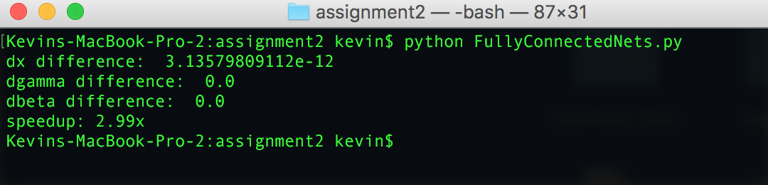
This version of the batchnorm backward pass can give you a significant boost in speed. I timed both versions and got a superb threefold increase in speed:

Conclusion

In this blog post, we learned how to use the chain rule in a staged manner to derive the expression for the gradient of the batch norm layer. We also saw how a smart simplification can help significantly reduce the complexity of the expression for dx. We finally implemented it the backward pass in Python using the code from CS231n. This version of the function resulted in a 3x speed increase!

If you’re interested in the staged computation method, head over to Kratzert’s nicely written post.

Cheers!